Unveiling Data Insights with Topological Analysis

1. Ben Fraser May 27, 2015 Persistent Homology in Topological Data Analysis

2. Data Analysis • Suppose we start with some point cloud data, and want to extract meaningful information from it

3. Data Analysis • Suppose we start with some point cloud data, and want to extract meaningful information from it • We may want to visualize the data to do so, by plotting it on a graph

4. Data Analysis • Suppose we start with some point cloud data, and want to extract meaningful information from it • We may want to visualize the data to do so, by plotting it on a graph • However, in higher dimensions, visualization becomes difficult

5. Data Analysis • Suppose we start with some point cloud data, and want to extract meaningful information from it • We may want to visualize the data to do so, by plotting it on a graph • However, in higher dimensions, visualization becomes difficult • A possible solution: dimensionality reduction

6. Principal Component Analysis • Essentially, fits an ellipsoid to the data, where each of its axes corresponds to a principal component

7. Principal Component Analysis • Essentially, fits an ellipsoid to the data, where each of its axes corresponds to a principal component • The smaller axes are those along which the data has less variance

8. Principal Component Analysis • Essentially, fits an ellipsoid to the data, where each of its axes corresponds to a principal component • The smaller axes are those along which the data has less variance • We could discard these less important principal components to reduce the dimensionality of the data while retaining as much of the variance as possible

9. Principal Component Analysis • Essentially, fits an ellipsoid to the data, where each of its axes corresponds to a principal component • The smaller axes are those along which the data has less variance • We could discard these less important principal components to reduce the dimensionality of the data while retaining as much of the variance as possible • Then may be easier to graph: identify clusters

10. Principal Component Analysis • Done by computing the singular value decomposition of X (each row is a point, each column a dimension):

11. Principal Component Analysis • Done by computing the singular value decomposition of X (each row is a point, each column a dimension): • Then a truncated score matrix, where L is the number of principal components we retain:

12. Principal Component Analysis • 8-dim data → 2-dim to locate clusters:

13. Principal Component Analysis • 3-dim → 2-dim collapses cylinder to circle:

14. Principal Component Analysis • Scale sensitive! Same transformation produces poor result on same shape/different scale data

15. Data Analysis • One weakness of PCA is its sensitivity to the scale of the data

16. Data Analysis • One weakness of PCA is its sensitivity to the scale of the data • Also, it provides no information about the shape of our data

17. Data Analysis • One weakness of PCA is its sensitivity to the scale of the data • Also, it provides no information about the shape of our data • We want something insensitive to scale which can identify shape (why?)

18. Data Analysis • One weakness of PCA is its sensitivity to the scale of the data • Also, it provides no information about the shape of our data • We want something insensitive to scale which can identify shape (why?) • Because “data has shape, and shape has meaning” - Ayasdi (Gunnar Carlsson)

19. Topological Data Analysis • Constructs higher-dimensional structure on our point cloud via simplicial complexes

20. Topological Data Analysis • Constructs higher-dimensional structure on our point cloud via simplicial complexes • Then analyze this family of nested complexes with persistent homology

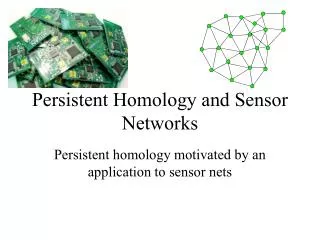
21. Topological Data Analysis • Constructs higher-dimensional structure on our point cloud via simplicial complexes • Then analyze this family of nested complexes with persistent homology • Display Betti numbers in graph form

22. Topological Data Analysis • Constructs higher-dimensional structure on our point cloud via simplicial complexes • Then analyze this family of nested complexes with persistent homology • Display Betti numbers in graph form • Essentially, we approximate the shape of the data by building a graph on it and considering cliques as higher dimensional objects, and counting the cycles of such objects.

23. Algorithm • Since scale doesn't matter in this analysis, we can normalize the data.

24. Algorithm • Since scale doesn't matter in this analysis, we can normalize the data. • Also, since we don't want to work with the entire data set (especially if it is very large), we want to choose a subset of the data to work with

25. Algorithm • Since scale doesn't matter in this analysis, we can normalize the data. • Also, since we don't want to work with the entire data set (especially if it is very large), we want to choose a subset of the data to work with • We would ideally like this subset to be representative of the original data (but how?)

26. Algorithm • Since scale doesn't matter in this analysis, we can normalize the data. • Also, since we don't want to work with the entire data set (especially if it is very large), we want to choose a subset of the data to work with • We would ideally like this subset to be representative of the original data (but how?) • This process is called landmarking

27. Landmarking • The method used here is minMax

28. Landmarking • The method used here is minMax • Start by computing a distance matrix D

29. Landmarking • The method used here is minMax • Start by computing a distance matrix D • Then choose a random point l1 to add to the subset of landmarks L

30. Landmarking • The method used here is minMax • Start by computing a distance matrix D • Then choose a random point l1 to add to the subset of landmarks L • Then choose each subsequent i-th point to add as that which has maximum distance from the landmark it is closest to:

31. Landmarking • The method used here is minMax • Start by computing a distance matrix D • Then choose a random point l1 to add to the subset of landmarks L • Then choose each subsequent i-th point to add as that which has maximum distance from the landmark it is closest to: li = p such that dist(p,L) = max{dist(x,L) ∀ x ϵ X} dist(x,L) = min{dist(x,l) ∀ l ϵ L}

32. Landmarking • Landmarking is not an exact science however: on certain types of data the method just used may result in a subset very unrepresentative of the original data. For example:

33. Algorithm • As long as outliers are ignored, however, the method used works well to pick points as spread out as possible among the data

34. Algorithm • As long as outliers are ignored, however, the method used works well to pick points as spread out as possible among the data • Next we keep only the distance matrix between the landmark points, and normalize it

35. Algorithm • As long as outliers are ignored, however, the method used works well to pick points as spread out as possible among the data • Next we keep only the distance matrix between the landmark points, and normalize it • This is all the information we need from the data: the actual position of the points is irrelevant, all we need are the distances between the landmarks, on which we will construct a neighbourhood graph

36. Neighbourhood Graph • Our goal is to create a nested sequence of graphs. To be precise, by adding a single edge at a time, between points x,y ϵ L, where dist(x,y) is the smallest value in D. Then replace the distance in D with 1.

37. Neighbourhood Graph • Our goal is to create a nested sequence of graphs. To be precise, by adding a single edge at a time, between points x,y ϵ L, where dist(x,y) is the smallest value in D. Then replace the distance in D with 1. • At each iteration of adding an edge, we keep track of r = dist(x,y), r ϵ [0,1]: this is our proximity parameter, and will be important when we graph the Betti numbers later.

38. Witness Complex Def: A point x is a weak witness to a p-simplex (a0,a1,...ap) in A if |x-a| < |x-b| ∀ a ϵ (a0,a1,...ap), and b ϵ A \ (a0,a1,...ap)

39. Witness Complex Def: A point x is a weak witness to a p-simplex (a0,a1,...ap) in A if |x-a| < |x-b| ∀ a ϵ (a0,a1,...ap), and b ϵ A \ (a0,a1,...ap) Def: A point x is a strong witness to a p-simplex (a0,a1,...ap) in A if x is a weak witness and additionally, |x-a0| = |x-a1| = … = |x-ap|.

40. Witness Complex Def: A point x is a weak witness to a p-simplex (a0,a1,...ap) in A if |x-a| < |x-b| ∀ a ϵ (a0,a1,...ap), and b ϵ A \ (a0,a1,...ap) Def: A point x is a strong witness to a p-simplex (a0,a1,...ap) in A if x is a weak witness and additionally, |x-a0| = |x-a1| = … = |x-ap| The requirement may be added that an edge is only added between two points if there exists a weak witness to that edge.

41. Simplicial Complexes • Next we want to construct higher dimensional structure on the neighbourhood graph: called a simplicial complex

42. Simplicial Complexes • Next we want to construct higher dimensional structure on the neighbourhood graph: called a simplicial complex • A simplex is a point, edge, triangle, tetrahedron, etc... (a k-simplex is a k+1-clique in the graph)

43. Simplicial Complexes • Next we want to construct higher dimensional structure on the neighbourhood graph: called a simplicial complex • A simplex is a point, edge, triangle, tetrahedron, etc... (a k-simplex is a k+1-clique in the graph) • A face of a simplex is a sub-simplex of it

44. Simplicial Complexes • Next we want to construct higher dimensional structure on the neighbourhood graph: called a simplicial complex • A simplex is a point, edge, triangle, tetrahedron, etc... (a k-simplex is a k+1-clique in the graph) • A face of a simplex is a sub-simplex of it • A simplicial k-complex is a set S of simplices, each of dimension ≤ k, such that a face of any simplex in S is also in S, and the intersection of any two simplices is a face of both of them

45. Simplicial Complexes • At each iteration, we add an edge: all we need to do is see if that creates any new k-simplices

46. Simplicial Complexes • At each iteration, we add an edge: all we need to do is see if that creates any new k-simplices • The edge itself adds a single 1-simplex to the complex

47. Simplicial Complexes • At each iteration, we add an edge: all we need to do is see if that creates any new k-simplices • The edge itself adds a single 1-simplex to the complex • A k-simplex is formed if the intersection of neighbourhoods of a k-2 simplex contains the two points in the added edge

48. Simplicial Complexes • At each iteration, we add an edge: all we need to do is see if that creates any new k-simplices • The edge itself adds a single 1-simplex to the complex • A k-simplex is formed if the intersection of neighbourhoods of a k-2 simplex contains the two points in the added edge • In other words, if every point in a k-2 simplex is joined to the two points in the edge, then together they form a k-simplex

49. Boundary Matricies • Next we compute boundary matricies. Essentially, these store the information that k-1 simplices are faces of certain k simplices

50. Boundary Matricies • Next we compute boundary matricies. Essentially, these store the information that k-1 simplices are faces of certain k simplices • For instance, in a simplicial complex with 100 triangles and 50 tetrahedra, the 4th boundary matrix has 100 rows and 50 columns, with zeros everywhere except where the given triangle is a face of the given tetrahedron, where it is 1.