Download
1 / 5
50 likes | 82 Views
This tutorial guides you through the steps of fitting transfer functions in MATLAB System Identification Toolbox. From creating input vectors to comparing model responses, learn how to analyze system models effectively.

E N D
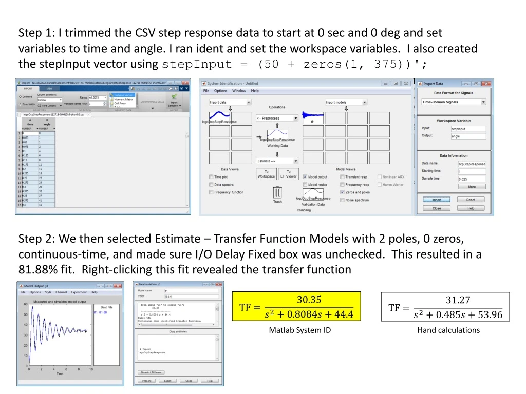
Step 1: I trimmed the CSV step response data to start at 0 sec and 0 deg and set variables to time and angle. I ran ident and set the workspace variables. I also created the stepInput vector using stepInput = (50 + zeros(1, 375))'; Step 2: We then selected Estimate – Transfer Function Models with 2 poles, 0 zeros, continuous-time, and made sure I/O Delay Fixed box was unchecked. This resulted in a 81.88% fit. Right-clicking this fit revealed the transfer function Matlab System ID Hand calculations
Step 3: Matlab System ID called fit tf1. Used pole(tf1) to determine poles Hand calculations Matlab System ID Poles = Poles =
Scope output for fitted DCP model simulinkDcpStepInputFittedModel112818a.slx 11/12/18 Evernote results i.e. hand-derived DCP model response. Compared to figure on the left, this model doesn’t match as well Overlay of CSV file (red) on simulated output
Scope output for fitted DCP model with PID simulinkDcpPidFittedModel112818a.slx 10/26/18 Evernote results i.e. hand-derived DCP model response Not too much difference… Overlay of CSV file (red) on simulated output
Scope output for fitted DCP model with PID FILE: legoDcpPolePlacementFittedModel1_0.slx 00courses\...\labview-XX-MatlabSystemId\legoDcpPolePlacementGains1_0.m