Download
1 / 20
340 likes | 997 Views
Diffusion (continued). Lecture 17. Fick’s First Law. Last time we derived Fick’s First Law. Continuity Equation. Imagine a volume and a flux of a species into that volume, J x , at X and a flux out, J x+dx , at x+dx .

E N D
Diffusion (continued) Lecture 17
Fick’s First Law Last time we derived Fick’s First Law
Continuity Equation • Imagine a volume and a flux of a species into that volume,Jx, at X and a flux out, Jx+dx, at x+dx. • Suppose nxatom/sec at x and nx+dxatoms/sec pass through the plane at x+dx. • The fluxes at the two planes are Jx= nx/dx2-sec and Jx+dx = nx+dx/dx2-sec. • Conservation of mass dictates that the increase in the number of atoms, dn, within the volume is just what goes in minus what comes out. • Over an increment of time dt this will be dn = (Jx-Jx+dx)dt.The concentration change is or: At fixed t and x
Deriving Fick’s Second Law • Continuity equation relates any change in flux along the gradient to change in concentration with time. • Since: • we have:
Fick’s Second Law • The second law says that the change in concentration with time at some point on a conc. gradient depends on the second derivative of the concentration gradient. • The straight line (∂2c/∂x2) is the steady state case. It is also the situation towards which a system will evolve over time.
Solutions to the Second Law • There is no ‘solution’ to the second law, rather there are a variety of solutions that depend on the boundary conditions of a particular situation. • As a first example, consider a thin layer (e.g., Ir at K-T boundary) of material at x = 0 at t = 0. These, together with mass conservation, are our boundary conditions. • Mass conservation is
Thin Flim Solution • Boundary conditions were x = 0 at t = 0 and • Solution, from Crank (1975), fitting these conditions is: • If diffusion can occur only in one direction:
Adjacent Layers • Now suppose with have one layer with concentration co abutting a second with c=0. • Crank’s solution is to superimpose the solutions for an infinite number of thin flims, dξ, and to sum their contributions to the total concentration at Xp. • Solution is:
Adjacent Layers • The solution to: • is • where erf is the error function and has the approximate form: • also available as the ERF function in Excel.
Other examples • Book has several other examples such as diffusion of Ni in a spherical, zoned olivine crystal with an initially homogeneous conc. of 2000 ppm and a conc. fixed at the rim by equilibrium with a magma at 500 ppm.
Diffusion in Multicomponents Systems • So far, we have considered only what is called traceror self diffusion - diffusion of a species who concentration is so small it has not affect on the system. • By definition, diffusion is a process in which there is no net transport across the boundary of interest (otherwise it is advection). Mass & charge balance require diffusion in one direction to be balanced by diffusion in another. • More generally, we can consider • Chemical diffusion • Multicomponent diffusion • Multicomponent chemical diffusion
Chemical Diffusion • Chemical diffusion refers to non-ideal situations where for one reason or another (e.g., medium is inhomogeneous, or diffusing species affects behavior of medium) we replace concentration with the chemical potential gradient. • where L is the chemical or phenomenological coefficient
Multicomponent Diffusion • This is where the concentration of an species is great enough that its diffusion depends on the diffusion of another species, e.g., Fe and Mg in ferromagnesian silicates (these elements tend to occupy the same site, so Mg can move in only if Fe moves out, etc). • Di,kis called the interdiffusion coefficient and computed as: • where n’s are the mole fractions. • The total solution is J = -DC (minus sign missing in book) • where J and C are (vertical) vectors of species and D is a matrix.
Multicomponent Chemical • Multicomponent chemical diffusion is a combination of the latter two, where we use interdiffusion coefficients and chemical potential. • Diffusion matrix is: J = -LC • Watson’s experiments dissolving quartz in basalt show an example where chemical diffusion must be used - note Na and K diffusing up a concentration gradient!
Mechanisms of Diffusion in Solids • Exchange: low probability • Interstitial: pretty much limited to He, etc. • Interstitiality: also low probability • Vacancy: most likely • Diffusion will then depend on both the probability of a jump and the probability of a vacancy. • Vacancies will increase with T: • where k is a rate constant and EH and activation energy for vacancy creation.
Diffusion Rates • Probability of atom making a jump to vacancy is • where ℵ is number of attempts and EB is the activation or barrier energy. • Combining, total diffusion rate will be product of probability. of a vacancy times probability of a jump: • where m and n are constants • At higher T, thermal vacancies dominate and • Bottom line: like other things in kinetics, we expect diffusion rates to increase exponentially with temperature.
Diffusion Rates • In general, the temperature of the diffusion coefficient is written as: • In log form: • At lower temperature, where permanent vacancies dominate, we might see different behavior because:
Determining Diffusion Coefficients • In practice, one would do a experiments at a series of temperatures with a tracer, determine the profile, solve Fick’s second law for each T. • Plotting ln D vs 1/T yields Do and EB. • Diffusion coefficient is different for each species in each material. • Larger, more highly charged ions diffuse more slowly.
Reactions at Surfaces Homogeneous reactions are those occurring within a single phase (e.g., an aqueous solution). Heterogeneous reactions are those occurring between phases, e.g., two solids or a solid and a liquid. Heterogeneous reactions necessarily occur across an interface.
Interfaces, Surfaces, and partial molar area • By definition, an interface is boundary between two condensed phases (solids and liquids). • A surface is the boundary between a condensed phase and a gas (or vacuum). • In practice, surface is often used in place of interface. • We previously defined partial molar parameters as the change in the parameter for an infinitesimal addition of a component, e.g., vi = (∂V/∂n)T,P,nj. We define the partial molar area of phase ϕ as: • where nis moles of substance. • Unlike other molar quantities, partial molar area is not an intrinsic property of the phase, but depends on shape, size, roughness, etc.For a perfect sphere: