Download
1 / 26
260 likes | 383 Views
Progression and propagation of internet congestion. Jim Gast University of Wisconsin / Madison Feb 19, 2002. When are losses likely?. When queuing delay is high? When queuing delay is rising fast? When queuing delay levels off? Randomly?. Queuing delay component in milliseconds. Time.

E N D
Progression and propagation of internet congestion Jim Gast University of Wisconsin / Madison Feb 19, 2002 jgast@cs.wisc.edu
When are losses likely? • When queuing delay is high? • When queuing delay is rising fast? • When queuing delay levels off? • Randomly? Queuing delay component in milliseconds Time jgast@cs.wisc.edu
Research Question • What are the characteristics of congestion in the Internet? • Duration • Propagation /location • Complexity • Frequency / periodicity • Implications jgast@cs.wisc.edu
Challenges • Accurately recreating congestion in the lab • multiple bottlenecks, appropriate length paths • Visualizing congestion to gain understanding • choosing the right level of detail (router vs. AS) • Inferring congestion from data we can realistically gather • passive vs. active • packet headers vs. flow level jgast@cs.wisc.edu
Your fair share 300 800 400 1100 800 1200 400 Assume 4 flows through 3 links. Each flow can support speeds up to 1000 packets per second. jgast@cs.wisc.edu
Your fair share At time t1, the blue flow ends. 300 0 800 400 1100 800 1200 400 800? When one of the flows ends, there is reduced congestion at the link with capacity 800. After t1, the black flow slowly increases toward 800 pps. jgast@cs.wisc.edu
Your fair share 300 600? 0 800 400 1100 800 1200 800 600? Increased flow of black packets causes congestion at the middle link. It responds by randomly dropping brown and black packets until the sum of brown and black drops to 1200. jgast@cs.wisc.edu
Your fair share 300 500? 600? 0 800 400 1100 800 1200 800 600? Congestion at the right link disappears. Decreased flow of brown packets leaves more room for green so green’s usage slowly rises toward 500 pps. jgast@cs.wisc.edu
Queue Depths Full … Empty Demand 70 74 78 96 100 104 70 Assume many flows converge at a particular link of capacity 100 packets per second. When aggregate demand exceeds 100,the queue starts to build. When the queue fills, the router dropspackets. Sometime later the senders learn about the loss, slowdown, and the queue length plummets. jgast@cs.wisc.edu
Time Frames Full Empty … 1 3 2 1 – No loss. Duration based on multiplexing factor, connection durations, RTT mix. Typ? 30 seconds to 30 minutes? 2 – Increasing queuing delay. Duration based on queue size, multiplexing, conn duration. Typ? 3 seconds to 10 seconds? 3 – Congestion event. Duration depends on shortest RTT plus three triple dup acks. Typ? 100 millisec to 300 millisec. jgast@cs.wisc.edu
Cascaded delays and congestion • Cumulative queuing delay will show brief periods ofelevated delay followed by a congestion event • Events will be spaced at seemingly random times,but with a period equal to the product of the periodsof the individual sites. jgast@cs.wisc.edu
Cascaded delays and risk of losses (Red lines = risk of loss from links A or B) Queue Depth Link A Time + Link B + Link C + Link D = Total jgast@cs.wisc.edu
Delay Count Shelf depends on theslope of building andemptying regimes Count Sampled at random intervals Height dependson duration ofcongestion event Delay Time Delay underfed congested Routers don’t tell us queue depth each millisecond. We have to discover it by probing. building emptying jgast@cs.wisc.edu
Additional Delay Count Delay Time Delay Queues aren’t always completely empty. If light cross traffic arrives at Poisson intervals, the delay counts will show an exponential distribution. jgast@cs.wisc.edu
Count Delay Sum of Delays Count + = ? Delay Router 1 Router 2 jgast@cs.wisc.edu
Surveyor Data • One-way delay measurements • GPS time accuracy • Feb 1999 to Aug 2000 jgast@cs.wisc.edu
Full Queue? • Zoom jgast@cs.wisc.edu
Level Shift jgast@cs.wisc.edu
Conceptual (unproven) Simulation 300 400 800 1100 800 1200 400 jgast@cs.wisc.edu
Next Steps • Wavelet Analysis • External Measurements • NIMI • Surveyor • WAWM • GIMI jgast@cs.wisc.edu
Implications • Improved tuning and performance of existing protocols • RED • ECN • Fewer surprises when the next killer app hits campus • Basis for cross-protocol next generation congestion control primitives • Lossless congestion control • Reduced delay, reduced jitter, reduced retransmissions when sharing • Improved Internet fairness, predictability, and scalability jgast@cs.wisc.edu
Questions? jgast@cs.wisc.edu
Simple bottleneck - pacing losses jgast@cs.wisc.edu
Multiple Congestion Disruptive Losses Disruptive Loss Desired Signal jgast@cs.wisc.edu
Analysis Example Disruptive Losses jgast@cs.wisc.edu
Shared Congestion Suspicion Total of congestion reports from all of the connections that pass through this site Component contributed by the connection in the prior slide jgast@cs.wisc.edu