Download
1 / 17
170 likes | 305 Views
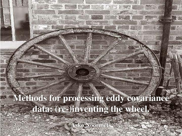
Methods for processing eddy covariance data: (re-)inventing the wheel. Asko Noormets. OUT Fluxes 0.000556 Hz data of Fc (carbon flux) LE (water flux) Hs (sensible heat flux). IN Measurements 10 Hz data of 3D wind speed T sonic H 2 O CO 2 Pressure. Processing.

E N D
Methods for processing eddy covariance data: (re-)inventing the wheel. Asko Noormets
OUT • Fluxes • 0.000556 Hz data of • Fc (carbon flux) • LE (water flux) • Hs (sensible heat flux) IN Measurements 10 Hz data of • 3D wind speed • Tsonic • H2O • CO2 • Pressure Processing
Theoretical assumptions (D. Baldocchi, J. Finnigan et al.) • Conservation of mass, i.e. input+output+storage=0 • Reynolds’ decomposition • Averaging done over long enough period (accommodate larger eddies), and over short enough periods (not be affected by diurnal patterns)
I II III IV Flux = change in mixing ratio (I) + advection (II) + flux divergence (vertical, lateral & longitudinal) (III) + biological source/sink strength (IV) Ideally: I=0, II=0, III=0 In reality: I II III 0 Measured covariance = true covariance + sensor bias
* * * * * * * Processing steps (D. Billesbach) 1. Replace spikes (>6) with the moving window mean. 2. Correct sonic temperature (CSAT) for humidity & pressure (IRGA). 3. Calculate deviations of each measurement from a 30-minute block average. 4. Calculate rotation angles using the block means (vmean = 0; wmean = 0). 5. Calculate all possible covariance pairs and rotated covariances. 6. Calculate density correction terms for LE and Fc (WPL). 7. Calculate the frequency correction factor for the sonic anemometer. 8. Calculate the frequency correction factor for the sonic anemometer and IRGA combination. 9. Adjust the WPL H term by the sonic frequency correction factor. 10. Adjust Fc and the WPL LE terms by the sonic-IRGA frequency correction factor. 11. Calculate final LE and Fc, that are rotated, adjusted for density and frequency bias.
Rotation: w v a b u Coordinate rotation
Fc+wpl+storage, July - w/o rotation - rotated
Fc+wpl+storage, November - w/o rotation - rotated
July Respiration, with () and without () coordinate rotation November
July Rotation effect (rerel): - uncorrected flux - wpl-corrected - wpl- & storage-corrected, gapfilled November
AQ parameters, MHW - w/o rotation - rotated
Uncertainties remain Flux = change in concentration (I) + advection (II) + flux divergence (vertical, lateral & longitudinal) (III) + biological source/sink strength (IV) Ideally: I=0, II=0, III=0 In reality: I II III 0 Measured covariance = true covariance + sensor bias (high- and low-pass filtering spectral correction factors 1.04-1.36 for Fc and LE)
For more comprehensive overview: Finnigan JJ, Clement R, Malhi Y, Leuning R, Cleugh HA (2003) A re-evaluation of long-term flux measurement techniques - Part I: Averaging and coordinate rotation. Boundary-Layer Meteorology107, 1-48.