Download
1 / 31
310 likes | 447 Views
Scheduling. Wayne Wolf Dept. of EE Princeton University wolf@princeton.edu. Outline. Review. Varieties of scheduling. Static scheduling. Feasibility. Scheduling algorithms. Reactive systems. Respond to external events. Engine controller. Seat belt monitor.

E N D
Scheduling Wayne Wolf Dept. of EE Princeton University wolf@princeton.edu
Outline • Review. • Varieties of scheduling. • Static scheduling. • Feasibility. • Scheduling algorithms.
Reactive systems • Respond to external events. • Engine controller. • Seat belt monitor. • Requires real-time response. • System architecture. • Program implementation. • May require a chain reaction among multiple processors.
Real-time systems • Perform a computation to conform to external timing constraints. • Deadline frequency: • Periodic. • Aperiodic. • Deadline type: • Hard: failure to meet deadline causes system failure. • Soft: failure to meet deadline causes degraded response. • Firm: late response is useless but some late responses can be tolerated.
Why scheduling? • The CPU is often shared among several processes. • Cost. • Energy/power. • Physical constraints. • Someone must be responsible for giving the CPU to processes. • Co-operation between processes. • RTOS.
Why CPU scheduling is not like hardware scheduling • Large variation in run times. • Asynchronous system architecture—no global clock to control processes. • Larger data-dependent variations in run time, coupled with greater desire to take advantage of slack times. • Processes may have variable start times.
Processes • A process is a unique execution of a program. • Several copies of a program may run simultaneously or at different times. • A process has its own state: • registers; • memory. • The operating system manages processes.
Timing requirements on processes • Period: interval between process activations. • Rate: reciprocal of period. • Initiation time: time at which process becomes ready. • Deadline: time at which process must finish.
Process characteristics • Process execution time Ti. • Execution time in absence of preemption. • Possible time units: seconds, clock cycles. • Worst-case, best-case execution time may be useful in some cases. • Sources of variation: • Data dependencies. • Memory system. • CPU pipeline.
A process can be in one of three states: executing on the CPU; ready to run; waiting for data. State of a process executing gets data and CPU gets CPU preempted needs data gets data ready waiting needs data
The scheduling problem • Can we meet all deadlines? • Must be able to meet deadlines in all cases. • How much CPU horsepower do we need to meet our deadlines?
Scheduling metrics • CPU utilization: • Fraction of the CPU that is doing useful work. • Often calculated assuming no scheduling overhead. • Utilization: • U = [ St1 ≤ t ≤ t2 T(t) ] / [t2 – t1]
Scheduling feasibility • Resource constraints make schedulability analysis NP-hard. • Must show that the deadlines are met for all timings of resource requests. P1 P2 I/O device
Simple processor feasibility • Assume: • No resource conflicts. • Constant process execution times. • Require: • T ≥ Si Ti • Can’t use more than 100% of the CPU. T1 T2 T3 T
Hyperperiod • Hyperperiod: least common multiple (LCM) of the task periods. • Must look at the hyperperiod schedule to find all task interactions. • Hyperperiod can be very long if task periods are not chosen carefully.
Hyperperiod example • Long hyperperiod: • P1 7 ms. • P2 11 ms. • P3 15 ms. • LCM = 1155 ms. • Shorter hyperperiod: • P1 8 ms. • P2 12 ms. • P3 16 ms. • LCM = 96 ms.
Simple processor feasibility example • P1 period 1 ms, CPU time 0.1 ms. • P2 period 1 ms, CPU time 0.2 ms. • P3 period 5 ms, CPU time 0.3 ms.
P Cyclostatic/TDMA • Schedule in time slots. • Same process activation irrespective of workload. • Time slots may be equal size or unequal. T1 T2 T3 T1 T2 T3 P
PLCM TDMA assumptions • Schedule based on least common multiple (LCM) of the process periods. • Trivial scheduler -> very small scheduling overhead. P1 P1 P1 P2 P2
TDMA schedulability • Always same CPU utilization (assuming constant process execution times). • Can’t handle unexpected loads. • Must schedule a time slot for aperiodic events.
TDMA schedulability example • TDMA period = 10 ms. • P1 CPU time 1 ms. • P2 CPU time 3 ms. • P3 CPU time 2 ms. • P4 CPU time 2 ms.
P Round-robin • Schedule process only if ready. • Always test processes in the same order. • Variations: • Constant system period. • Start round-robin again after finishing a round. T1 T2 T3 T2 T3 P
Round-robin assumptions • Schedule based on least common multiple (LCM) of the process periods. • Best done with equal time slots for processes. • Simple scheduler -> low scheduling overhead. • Can be implemented in hardware.
Round-robin schedulability • Can bound maximum CPU load. • May leave unused CPU cycles. • Can be adapted to handle unexpected load. • Use time slots at end of period.
Priority-driven scheduling • Each process has a priority. • CPU runs the highest-priority process that is ready. • Priorities determine scheduling policy: • fixed priority; • time-varying priorities.
Priority-driven scheduling example • Rules: • each process has a fixed priority (1 highest); • highest-priority ready process gets CPU; • process continues until done. • Processes • P1: priority 1, execution time 10 • P2: priority 2, execution time 30 • P3: priority 3, execution time 20
P3 ready t=18 P2 ready t=0 P1 ready t=15 Priority-driven scheduling example P2 P1 P2 P3 30 60 0 10 20 40 50 time
Priority-driven schedulability • Depends on priorities: • Dynamic vs. static. • Relationship to process execution times. • Results depend on discipline: • RMS. • EDF.
Schedulability and CPU selection • How fast a CPU do we need to make our system of processes schedulable? • Process execution time depends on CPU. • Ideal case: process execution time scales linearly.
Non-idealities in process scaling • Within a single CPU model: • Memory speed doesn’t scale with CPU speed. • Across CPU models: • Pipeline delays may vary. • Memory system, etc.
Example: Space Shuttle software error • Space Shuttle’s first launch was delayed by a software timing error: • Primary control system PASS and backup system BFS. • BFS failed to synchronize with PASS. • Change to one routine added delay that threw off start time calculation. • 1 in 67 chance of timing problem.