Lecture 3 Laplace transform

1. Physics for informatics Lecture 3Laplace transform Ing. Jaroslav Jíra, CSc.

2. The Laplace transform What is it good for? • Solving of differential equations • System modeling • System response analysis • Process control application

3. The Laplace transform Solving of differential equations procedure A system analysis can be done by several simple steps • Finding differential equations describing the system • Obtaining the Laplace transform of these equations • Performing simple algebra to solve for output or variable of interest • Applying inverse transform to find solution

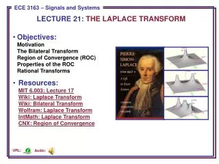
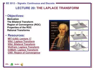
4. The Laplace transform The definition • The Laplace transform is an operator that switches a function of real variable f(t) to the function of complex variable F(s). • We are transforming a function of time - real argument t to a function of complex angular frequency s. • The Laplace transform creates an image F(s) of the original function f(t) where s= σ+ iω

5. The Laplace transform Restrictions • The function f(t) must be at least piecewise continuous for t ≥ 0. • |f(t)| ≤ Meαt where M and α are constants. The function f(t) must be bounded, otherwise the Laplace integral will not converge. • We assume that the function f(t) = 0 for all t < 0

6. The Laplace transform Inverse Laplace transform • Inverse transform requires complex analysis to solve • If there exists a unique function F(s)=L[f(t)], then there is also a unique function f(t)=L-1[F(s)] • Using the previous statement, we can simply create a set of transform pairs and calculate the inverse transform by comparing our image with known results in time scope

7. The Laplace transform Basic properties Linearity Scaling in time Time shift Frequency shift

8. The Laplace transform Another properties

9. The Laplace transform The most commonly used transform pairs

10. The Laplace transformTransform pair deduction u(t) 1 Unit step The unit step u(t) is defined by t 0 The Laplace image u(t) Shifted unit step 1 t 0 a The Laplace image

11. The Laplace transformTransform pair deduction f(t) Unit impulse 1/t1 The unit impulse f(t) is characterized by unit area under its function t 0 t1 The Laplace image f(t) Dirac delta It is a unit impulse for t1→ 0 t 0

12. The Laplace transformTransform pair deduction Exponential function Linear function Per partes integration

13. The Laplace transformTransform pair deduction Square function Per partes integration The n-th power function

14. The Laplace transformTransform pair deduction Cosine function Sine function

15. The Laplace transformTransform pair deduction Time shift f(t) f(t-a) The original function f(t) is shifted in time to f(t-a) t 0 a Frequency shift

16. The Laplace transformProperty deduction Time differentiation Per partes integration

17. The Laplace transformProperty deduction Per partes integration Time integration

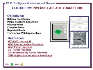
18. Inverse Laplace transform The algorithm of inverse Laplace transform Since the F(s) is mostly fractional function, then the most important step is to perform partial fraction decomposition of it. Depending on roots in denominator, we are looking for the following functions, where A and B are real numbers:

19. Inverse Laplace transformBasic examples of partial fraction decomposition to find the original f(t) Two distinct real roots The equation s2+4s +3= 0 has two distinct real roots s1= -3 and s2= -1 We have to find coefficients A and B for Multiplying the equation by its denominator Now we can substitute Decomposed F(s) so the original function

20. Inverse Laplace transform One real root and one real double root The denominatorhas a single root s1= -1 and a double root s23= -3 We are looking for coefficients A,Band C Multiplying the equation by its denominator Now we can substitute to get A,B; the C coefficient can be obtained by comparison of s2factors Decomposed F(s) so the original function

21. Inverse Laplace transform Two pure imaginary roots Since we know, that it will be helpful to rearrange the original formula Now we can directly write the result

22. Inverse Laplace transform One real root and two pure imaginary roots We are looking for coefficients A,Band C Multiplying the equation by its denominator Now we can substitute to get A; B,Ccoefficients can be obtained by comparison of s0,s2factors Decomposed F(s) so the original function

23. Inverse Laplace transform Two complex conjugated roots We have to rearrange the denominator in the first step Decomposed F(s) Now we have to assemble all necessary relations so the original function

24. Solving of differential equations by the Laplace transform Example 1 Find the x(t) on the interval <0,∞) The image of desired function is From the former definitions we know, that Then we can write The original function

25. Solving of differential equations by the Laplace transform Example 2 Function on the right side Necessary relations Equation in the Laplace form

26. Solving of differential equations by the Laplace transform Example 2- continued A formula for the X(s) after the partial fraction decomposition after some small arrangements The original function

27. Solving of differential equations by the Laplace transform Example 3 Homogeneous second order LDR Necessary relations Equation in the Laplace form The original function

28. Solving of differential equations by the Laplace transform Example 4 Inhomogeneous second order LDR Necessary relations Equation in the Laplace form knowing that The original function

29. Solving of differential equations by the Laplace transform Example 5 Integro-differential equation Necessary relations Equation in the Laplace form The original function