Download
1 / 51
510 likes | 526 Views
The paper discusses a parallel algorithm for the single-source shortest path problem on planar digraphs, utilizing concepts like Dijkstra's algorithm and parallel processing. The presentation includes a detailed explanation with accompanying illustrative examples.

E N D
A Simple Parallel Algorithm for the Single-Source Shortest Path Problem on Planar Digraphs Authors:Jesper L. Traff and Christos D. Zaroliagis Citation:Journal of Parallel and Distributed Computing. Vol. 60, Issure 9, Sep. 2000, pp 1103-1124. Presented by Beifang Yi
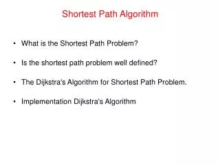
About presentation 1. Introduction 2. The parallel algorithm 3. Other algorithms needed for this so-called simple implementation
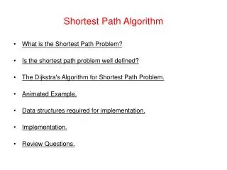
What is the shortest path problem? Crazy Question ?
The shortest path?Yes! Our dog does a good job, by intuition.
But onto this intuition, • We Human Beings spreada bunch of conceited, snobbish, mind-splitting, glittering glazes, such as: • Direction (a path has direction), • Weight or cost of a path… and … • Digraph.
To strength our advantage over the animal, • We further borrow an item “ planar” to meddle with the relative simple “Digraph”. • Planar graph: it can be drawn on a plane so that the edges intersectonly at the vertices.
for example, • In the first 5 complete graphs, the first 4 are planar graphs, but K5 is not.
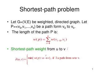
Legs in another stubborn, mulish phrase: ssspp • i.e. single-source shortest pathproblem: • To find shortest paths (tree) from a given source vertex to every other vertex in G.
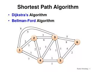
To our temporary relief, • A guy called Dijkstra intruded in the arena, picking up the dog’s intuition: • Find from the limited connected points the nearest point, and remove it into the sought set of points.
Dijkstra’s algorithm operation: http://ciips.ee.uwa.edu.au/~morris/Year2/PLDS210/dij-op.html From :
Initial graphAll nodes have infinite cost except the source Dijkstra’s algorithm:
Choose the closest node to s. As we initialised d[s] to 0, it's s. Add it to S Relax all nodes adjacent to s. Update predecessor (red arrows) for all nodes updated. Dijkstra’s algorithm:
Choose the closest node, x Relax all nodes adjacent to x Update predecessors for u, v and y. Dijkstra’s algorithm:
Now y is the closest, add it to S. Relax v and adjust its predecessor Dijkstra’s algorithm:
u is now closest, choose it and adjust its neighbour, v. Dijkstra’s algorithm:
Finally, add v. The predecessor list now defines the shortest path from each node to s. Dijkstra’s algorithm:
To our dismay: The authors of this paper tried to manipulate Dijkstra’s initiative to crack ssspp in the showy, brassy Parallel stadium, not a good performing stage for ssspp.
Even worse: They used one of the dullest, most strident languages, mathematical jargon, to portray their deliberation.
So, I have to add some spicy seasoning in the process of interpreting their boring, mind-numbing essay: -----by using exemplar pictures.
pizza 2’: We divide G into 3 regions (R1-3) such that: Source V1 is in R1, Interior vertices (circled ones), Boundary vertices (round rectangles), shared among atleast 2 regions, No edges between 2 interior vertices in different regions.
For boundary Vs (as the source vertices), find in parallel the single shortest path trees. e.x. Vj keeps 7 shortest paths (because of 7 boundary vertices). (Sequential Dijkstra’s). Pizza 3: Shortest paths in every region.
If source V1 is not a boundary vertex of R1, solve the ssspp inside R1 with source vertex V1; Else: skip this step. Pizza 4: Shortest paths in region 1.
Pizza 5: Contraction of G into G’ • Vertices of G’: source V1 and all boundary vertices of G; • Add an edge between any two boundary vertices in the same Ri with weight equal to the distance in Ri (calculated in step 2 or 3). • Consider V1 as a boundary vertex.
Pizza 5: The shortest path tree in G’ • Find the shortest path tree in G’ rooted as source V1; • Using parallel Dijkstra’s algorithm.
Pizza 6: Shortest path tree in G • for each interior vertexu in Ri, • in parallel for every boundary Vb in Ri, find the minimum distance of V1 to u through Vb, while recording the parent of u.
Pizza 6’: Shortest path tree Ts in G • Distances from V1to every boundary vertex ub have been computed in previous step, so only the parent pb of ub needs to be updated if necessary. • We have to consider some trivial cases: pb and ub are in the same Ri? pb= V1? pb is a boundary vertex?
Pizza 6”: Shortest path tree Ts in G • In this step 6, one special case: if V1 is not a boundary vertex. • The distance and parent information for the interior vertices in R1 needs to be updated with that obtained in step 4.
? How to divide G ? Because of time limit, I could only cook one piece of tasteless bland cookiefor this part.
Piece 1: Separator A separator of a graph (V, E): a subset C of V whose removal partitions V into 2 disjoint A, B, such that any path from a vertex in A to a vertex in B contains at least one vertex from C.
Piece 2: Planar separator theorem G=(V,E): an n-vertex planar graph with nonnegative costs on its vertices summing up to one a separator S partitions V into 2 sets V1, V2, such that |S|=O(n1/2) and V1, V2 has total cost at most 2/3 each.
Piece 3: r-Division A region decomposition of G into O(n/r) regions such that each region has at most c1r vertices and at most c2 r1/2 boundary vertices.
Piece 4: Decomposition of G Recursively applying the planar separator theorem. Doing BFS (breadth first search) from V1: all vertices at any level/depth make up a separator!
Piece 5: The most insipid piece The authors here present an “explicit” EREW PRAM implementation of Frederickson’s algorithm by using
Piece 5’: The most insipid piece Gazit—Miller separator algorithm, which is a “clever” parallelization of the sequential approachby
Piece 6: The most insipid piece Lipton and Tarjan. After painstakingly sketching those schemes, the authors conclude:
Piece 7: Finally, finale “Our algorithm runs in O((n2e + n1-e)log n) time and performs (n1+elog n) work on an EREW PRAM, for any 0<e<1/2.” And
Piece 7: Ending “Climax” ( A brag? Seems not) ssspp “can be solved in O(n2e + n1-e) time and performs (n1+e) work on an EREW PRAM”, if Sam’s sequential Dijkstra and John’s parallel Dijkstra are used!!!
Huh, … Thanks for patience! and Welcome for questions.