Download
1 / 11
110 likes | 243 Views
Limitation of COS S/N No good 2-D flat available. Fixed pattern noise dominates COS spectra. An uncalibrated COS spectrum is affected by: Optical response Smooth F ixed in wavelength space (sort of) Fixed pattern noise Due to detector irregularities

E N D
Limitation of COS S/N • No good 2-D flat available. • Fixed pattern noise dominates COS spectra. • An uncalibrated COS spectrum is affected by: • Optical response • Smooth • Fixed in wavelength space (sort of) • Fixed pattern noise • Due to detector irregularities • Rapidly varying with detector position • Fixed in detector space • Separating fixed pattern noise and spectrum: • Iterative approach • Direct approach COS signal to noise capabilities
Data taken at several, slightly shifted wavelengths • Align all of the spectra in λspace and create a mean spectrum (reduces fixed pattern noise by 1/√N). • Divide each spectrum by the mean and average the results in detector space for an estimate of the fixed pattern noise. • Divide each spectrum by the fixed pattern noise estimate. • GOTO 1 and iterate “until done”. • Some limitations: • Algorithm can get “confused” by busy spectra. • COS FP-POS offsets are nearly identical, so some spatial frequencies are poorly constrained. • Works well in many cases, but error estimates are a bit sketchy. The FP-POS Algorithm
A1-D flat derived by the FP-POS algorithm, as implemented by Tom Ake for COS. Grid wire shadows are marked.
(Left) Net spectrum of WD0308-565 from FP-Split algorithm, binned by 3 pixels (half a RESOL). Also shown: 3 weak S II IS lines, and a quadratic fit to 1220 < λ < 1250 Å. (Upper right) Poisson S/N in each bin. Features are spectral lines or grid wires. (Right) Normalized S II spectrum showing how well weak lines can be identified.
To determine limiting S/N, need good error estimates for the fixed pattern template. • Uncalibrated standard stars typically have simple continua, whose line free regions can be represented by polynomials. • Align all spectra in wavelength space and fit them with one polynomial. • Divide each spectrum by the fit and average the results in detector space to get the fixed pattern noise. • No iteration needed. • Template errors follow from simple propagation of errors. • Some limitations: • Only works for sources with simple continua. • Agrees well with templates from iterative approach. The Direct Approach
Examples of polynomial fits Examples of fits to 4 FPPOS NET spectra from program 12086. Regions containing stellar lines (other than Ly α), IS lines and grid wire shadows have been eliminated. These high S/N data show how well polynomials fit the NET spectra.
Comparison of iterative and direct flats. Ratios of the NET spectra (black) and templates (red) -- both smoothed by 64 points to highlight systematic differences. Bluecurve is the average of the two ratios.
Portions of a 1-D flat showing ±1σ errors. Data are binned over 3 pixels, half a RESOL, and grid wire shadows are marked.
Histograms characterizing fixed pattern noise in each grating/detector. Plots show the dispersion about the mean of the fixed pattern templates including the grid wires (black), without grid wires (red) and expected Poisson errors (blue).
RMS S/N over the regions 1300 < x < 152000 for FUVA and 1000 < x < 145000 -- corrected for Poisson noise. The Bottom Line for Standard Processing • G130M is better than G160M because it’s fatter. • FUVB is better than FUVA because it is. • To improve, a full 1-D flat is needed. • A S/N = 50 template limits overall S/N to ≤ 100.