Download
1 / 25
250 likes | 921 Views
EARTHQUAKE SCIENCE-ENGINEERING INTERFACE: STRUCTURAL ENGINEERING RESEARCH PERSPECTIVE Allin Cornell Stanford University SCEC WORKSHOP Oakland, CA October, 2003. Objective. λ C = mean annual rate of State C , e.g., collapse

E N D
EARTHQUAKE SCIENCE-ENGINEERING INTERFACE: STRUCTURAL ENGINEERING RESEARCH PERSPECTIVE Allin Cornell Stanford University SCEC WORKSHOP Oakland, CA October, 2003
Objective • λC = mean annual rate of State C, e.g., collapse • Two Steps: earth science and structural engineering: λC = ∫PC(X) dλ(X) • Where X = Vector Describing Interface
“Best” Case • X = {A1(t1), A2(t2), …Ai(ti)..} for all ti = i∆t , i = 1, 2, …n i.e., an accelerogram ·dλ(x) = mean annual rate of observing a “specific” accelerogram, e.g., a(ti) < A(ti) <a(ti) + da for all ∙Then engineer finds PC(x) for all x ∙ Integrate
Current Best “Practice” (or Research for Practice) • λC = mean annual rate of State C, e.g., collapse • Two Steps: earth science and structural engineering: λC = ∫PC(IM) dλ(IM) • IM = Scalar “Intensity Measure”, e.g., PGA or Sa1 • λ(IM) from PSHA • PC(IM) found from “random sample” of accelerograms = fraction of cases leading to C
Current Best Seismology Practice*: ·Disaggregate PSHA at Sa1 at po, say, 2% in 50 years, by M and R: fM,R|Sa. Repeat for several levels, Sa11, Sa12, … · For Each Level Select Sample of Records: from a “bin” near mean (or mode) M and R. Same faulting style, hanging/foot wall, soil type, … · Scale the records to the UHS (in some way, e.g., to the Sa(T1)). *DOE, NRC, PEER, … e.g., see R.K. McGuire: “... Closing the Loop”( BSSA, 1996+/-); Kramer (Text book; 1996 +/-); Stewart et al. (PEER Report, 2002)
105 105 105 105 105 106 157 241 241 241 Seismic Design Assessment of RC Structures. (Holiday Inn Hotel in Van Nuys) • Beam Column Model with Stiffness • and Strength Degradation in Shear and Flexure • using DRAIN2D-UW by J. Pincheira et al.
Multiple Stripe Analysis C • The Statistical Parameters of the “Stripes” are Used to Estimate the Median and Dispersion as a Function of the Spectral Acceleration, Sa1.
Best “Research-for-Practice” (Cont’d) : • Analysis: λC = ∫PC(IM) dλ(IM) ≈ ∑PC(IMk) ∆ λ(IMk) • Purely Structural Engineering Research Questions: • Accuracy of Numerical Models • Computational Efficiency
Best “Research-for-Practice”: • Analysis: λC = ∫PC(IM) dλ(IM) ≈ ∑PC(IMk) ∆ λ(IMk) ·Interface Questions: What are good choices for IM? Efficient? Sufficient? How does one obtain λ(IM) ? How does one do this transparently, easily and practically?
BETTER SCALAR IM? More Efficient? IM = Sa1 IM = g(Sd-inelastic; Sa2) (Luco, 2002) • when IM1I&2E is employed in lieu of IM1E, (0.17/0.44)2 ≈ 1/7 the number of earthquake records and NDA's are needed to estimate a with the same degree of precision
Sa MAGNITUDE DRIFT Sa Van Nuys Transverse Frame: Pinchiera Degrading Strength Model; T = 0.8 sec. 60 PEER records as recorded 5.3<M<7.3.
DRIFT MAGNITUDE Residual-residual plot: drift versus magnitude (given Sa) for Van Nuys. (Ductility range: 0.3 to 6) (60 PEER records, as recorded.)
DRIFT MAGNITUDE Residual-residual plot: drift versus magnitude (given Sa) of a very short period (0.1 sec) SDOF bilinear system. (Ductility range 1to 20.) (47 PEER records, as recorded.)
DRIFT MAGNITUDE Residual-residual plot: drift versus magnitude (given Sa) for 4-second, fracturing-connection model of SAC LA20. Records scaled by 3. Ductility range: mostly 0.5 to 5
What Can Be Done That is Still Better? • Scalar to (Compact) Vector IM • Interface Issues: What vector? How to find λ (IM)? • Examples: {Sa1, M}, {Sa1, Sa2}, … ·PSHA: λ(Sa1, M) = λ(Sa1) f(M| Sa1) (from “Deagg”) λ(Sa1, Sa2) Requires Vector PSHA (SCEC project)
Vector-Based Response Prediction Vector-Valued PSHA
Future Interface Needs • Engineers: • Need to identify “good” scalar IMs and IM vectors. • In-house issues: what’s “wrong” with current candidates? When? Why? How to fix? • How to make fast and easy, i.e., professionally useful.
Future Interface Needs (con’t) • Help from Earth scientists: Guidance (e.g., what changes frequency content? Non-”random” phasing? ) · Earth Science problems:How likely is it? λ(X) • λ(X) = ∫P(X \ Y) dλ(Y) • X = ground motion variables (ground motion prediction: empirical, synthetic) • Y = source variables (e.g., RELM)
Future Needs(Cont’d) • Especially λ(X) for “bad” values of X (Or IM). ·Some Special Problems: Nonlinear Soils, Strong Directivity, Aftershocks, Spatial Fields of X.
DRIFT MAGNITUDE Residual-residual plot: drift versus magnitude (given Sa) for 4-second, fracturing-connection model of SACLA20. Ductility range: 0.2 to 1.5. Same records.
Non-Linear MDOF Conclusion: (Given Sa(T1) level) the median (displacement) EDP is apparently independent of event parameters such as M, R, …*. Implications: (1) the record set used need not be selected carefully selected to match these parameters to those relevant to the site and structure. Comments: Same conclusion found for transverse components. More periods and backbones and EDPs deserve testing to test the limits of applicability of this illustration. *Provisos: Magnitudes not too low relative to general range of usual interest; no directivity or shallow, soft soil issues.