Download

1 / 31
310 likes | 469 Views
HASE: A Hybrid Approach to Selectivity Estimation for Conjunctive Queries. Xiaohui Yu University of Toronto xhyu@cs.toronto.edu Joint work with Nick Koudas (University of Toronto) and Calisto Zuzarte (IBM Toronto Lab). Outline. Background Motivation Related Work HASE Estimator

E N D
HASE: A Hybrid Approach to Selectivity Estimation for Conjunctive Queries Xiaohui Yu University of Toronto xhyu@cs.toronto.edu Joint work with Nick Koudas (University of Toronto) and Calisto Zuzarte (IBM Toronto Lab)
Outline • Background • Motivation • Related Work • HASE • Estimator • Algorithms • Bounds • Experiments • Conclusions
Query Optimization • Execution plans differ in costs • Difference can be huge (1 sec vs. 1 hour) • Which Plan to Choose?? • Query Optimization • Estimate the costs of different plans • Choose the plan with the least cost • Cost Estimation • Factors: run-time environments, data properties, …
Selectivity • Important factor in costing: selectivity • Fraction of records satisfying the predicate (s) • E.g., 100 out of 10,000 records having salary > 3000 s = 100/10000 = 0.01 • Selectivity can make a big difference Plan 2: Index scan cost Cost = s * const2 Plan 1: Table scan Cost = const1 s = 0.01 Selectivity (s)
Related Work • Two streams • Synopsis-based • Sampling-based • Synopses • Capture the characteristics of data • Obtained off-line, used on-line • E.g., Histograms
Histograms 3000 A: # of records in red / total # of records Estimate = ( 500 + 800 + 1700 ) / 5000 = 0.6 1700 1000 1500 800 2500 3500 5000 6000 Salary Q: Selectivity of salary>3000?
Synopses: pros and cons • Pros: • Built offline; can be used many times • minimal overhead at selectivity estimation time • Cons: • Difficult to capture all useful information in a limited space • Correlation between attributes
Sampling Number of records in the table: 10,000 Sample size: 100 Number of records having age > 50 and salary > 5500 : 12 Selectivity estimate = 12/100 = 0.12 True selectivity = 0.09
Sampling: pros and cons • The good: • Provides correlation info through the sample • The bad: • Cost, cost… • Accurate results require a large portion of the data to be accessed • Random access is much slower than sequential access
Summary Take the best of both worlds? Capture correlation + reduce sampling rate
Outline • Background • Motivation • Related Work • Our approach: HASE • Estimator • Algorithms • Bounds • Experiments • Conclusions
HASE 1700 1000 1500 800 6000 2500 3500 5000 Salary • Hybrid approach to selectivity estimation Goal: Consistent utilization of both sources of information • Benefits: • Correlation is captured (sampling) • Sample size can be significantly smaller (histograms)
Problem setting Data: Table of size N • Conjuncts of predicates Q = P1^P2^P3 ^… • (age>50)^(salary>5500)^(hire_date>”01-01-05”) • P1 P2 P3 Query: • Selectivities of individual predicates (obtained from synopses)s1 = 0.1, s2 = 0.2, s3 = 0.05 • A Sample S of nrecords Inclusion probability of recordj : jFor simple random sampling (SRS) j= n/N Available info: Goal Estimate the selectivity sof the query Q
Example Table R with 10,000 records Query Q = P1^P2 on two attributes Suppose 500 records satisfy both predicates True Selectivity s = 500/10000 = 0.05
Histogram-based estimate Assuming independence between attributes Selectivity estimate Based on the histograms, s1 = 0.6, s2 = 0.3 Relative error = |0.18 – 0.05 | /0.05 = 260%
Sampling-based estimate Sample weightof j : dj = 1/ j Indicator variable Selectivity Estimate (HT estimator) Take a SRS of size 100 dj = 10000/100 = 100 9 records satisfy Q Estimate = 9*100/10000 = 0.09 Relative error = | 0.05 – 0.09 | / 0.05 = 80%
A new estimator Original weights Known selectivities (through histograms) s1, s2, … New weights Calibration estimator wj: (1) reproduce known selectivities of individual predicates (2) as close to dj as possible
Consistency with known selectivities Observed frequencies from sample 100 sample records from 10,000 records in the table dj = 100 s1 = 0.6
Calibration estimator Why do we want wj to be as close as djas possible? dj have the property of producing unbiased estimates Keep wj as close to dj as possible wj remain nearly unbiased
Constrained optimization problem Distance function D(x) (x = wj /dj ) (As close to dj as possible) w.r.t. wj Minimize Subject to (reproduce known selectivities) Yes: 1 j satisfies Pi? No: 0
An algorithm based on Newton’s method Method of Lagrange multipliers Minimize w.r.t. where Can be solved using Newton’s method via an iterative procedure. wj
Example Observed frequencies from sample
Distance measures • Requirements on the distance function(1) D is positive and strictly convex(2) D(1) = D’(1) = 0(3) D’’(1) = 1 • Linear function • only one iteration required fast! • wj< 0 possible negative estimates • Multiplicative function • Converges after a few iterations (typically two) • wj> 0 always
Error bounds • Probabilistic bounds = Pr ( both j and l are in the sample )
Experiments • Synthetic data • Skew: Zipfian distribution (z=0,1,2,3) • Correlation: corr. coef. between attributes: [0, 1] • Real data • Census-Income data from UCI KDD Archive • Population surveys by the US Census Bureau. • ~200,000 records, 40 attributes • Queries • Range queries: attribute<= constant • Equality queries: attribute = constant
Effect of number of attributes z = 0, correlation = 0.85, sample rate = 0.01 1.8 HASE 1.6 Sampling Synopsis 1.4 1.2 1 Absoluate relative error 0.8 0.6 0.4 0.2 0 2 2.5 3 3.5 4 4.5 5 Number of attributes
Conclusions Selectivity Estimation Synopsis-based estimation Sampling-based estimation HASE • The calibrated estimator • Algorithms • Probabilistic bounds on errors • Experimental results • Benefits: • Capturing correlation (sampling) • Sample size can be significantly smaller (histograms)