Download

1 / 16
180 likes | 401 Views
Discriminant Analysis. Defining and Testing Groups. Goals. Develop classificatory key for groups that have already been defined Identify important variables in defining clusters after cluster analysis Classify new observations into an existing classification. Two Approaches.

E N D
Discriminant Analysis Defining and Testing Groups
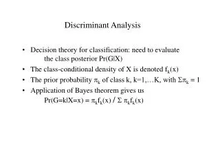
Goals • Develop classificatory key for groups that have already been defined • Identify important variables in defining clusters after cluster analysis • Classify new observations into an existing classification
Two Approaches • Discriminant Analysis – Assign probabilities of group membership to an unknown specimen • Canonical Discriminant Analysis – Display a picture of the groups in two dimensions using discriminant function scores
Steps • Need more cases than variables – preferably five more cases in each group than the number of variables • Explanatory variables are interval, ratio, or dichotomous • Response variable is nominal (categorical)
Analysis • Discriminant Analysis finds linear combination of the explanatory variables that provides the maximum separation of the group means • Subsequent dimensions must be orthogonal (uncorrelated) • The maximum number of dimensions is k-1 where k is the number of groups
Snodgrass Houses (Again) • Rcmdr does not provide access to discriminant analysis • lda() computes the functions • plot() plots the scores by group • predict() predicts group membership of original or new data
> LdaModel.1 <- lda(Inside~Area, prior=c(.5, .5), data=Snodgrass) > LdaModel.1 Call: lda(Inside ~ Area, data = Snodgrass, prior = c(0.5, 0.5)) Prior probabilities of groups: Inside Outside 0.5 0.5 Group means: Area Inside 317.3711 Outside 179.0566 Coefficients of linear discriminants: LD1 Area 0.01538446 > plot(LdaModel.1)
> PInside<- predict(LdaModel.1) > PInside > str(PInside) List of 3 $ class : Factor w/ 2 levels "Inside","Outside": 2 1 1 1 1... $ posterior: num [1:91, 1:2] 0.0319 0.5634 0.869 0.9987 0.995 ... ..- attr(*, "dimnames")=List of 2 .. ..$ : chr [1:91] "1" "2" "3" "4" ... .. ..$ : chr [1:2] "Inside" "Outside" $ x : num [1:91, 1] -1.603 0.12 0.889 3.127 2.489 ... ..- attr(*, "dimnames")=List of 2 .. ..$ : chr [1:91] "1" "2" "3" "4" ... .. ..$ : chr "LD1“ > xtabs(~Snodgrass$Inside+PInside$class) PInside$class Snodgrass$Inside Inside Outside Inside 29 9 Outside 5 48 > (29+48)/(29+9+5+48) [1] 0.8461538
Results • Predictions are the same as when we used logistic regression • Predictions are optimistic since we used the data to generate the model • Could split data – run lda() on one half and predict the other half • Could use cross-validation run lda() n times leaving one case out each time
> LdaModel.2 <- lda(Inside~Area, data=Snodgrass, + prior=c(.5, .5), CV=TRUE) > LdaModel.2 $class [1] Outside Inside InsideInsideInsideInsideInsideInside [9] Outside Outside Inside Outside OutsideOutside Inside Inside . . . $posterior Inside Outside 1 0.0329603669 0.9670396331 2 0.5703984220 0.4296015780 3 0.8664921383 0.1335078617 4 0.9988861784 0.0011138216 5 0.9950634758 0.0049365242 . . . > xtabs(~Snodgrass$Inside+LdaModel.2$class) LdaModel.2$class Snodgrass$Inside Inside Outside Inside 29 9 Outside 6 47 > (29+47)/(29+9+6+47) [1] 0.8351648
Segments • Expand the model to predict Segment (1, 2, 3) • Add variables Total and Types • Accuracy is 68% (against chance of 33%) Segment accuracy is 76%, 68%, and 56% for Segement 3
> LdaModel.3 <- lda(Segment~Area+Types+Total, data=Snodgrass, + prior=rep(1/3,3)) > LdaModel.3 Call: lda(Segment ~ Area + Types + Total, data = Snodgrass, prior = rep(1/3, 3)) Prior probabilities of groups: 1 2 3 0.3333333 0.3333333 0.3333333 Group means: Area Types Total 1 317.3711 7.684211 13.23684 2 166.7946 1.821429 2.00000 3 192.7900 1.680000 2.00000
Coefficients of linear discriminants: LD1 LD2 Area -0.01138796 0.01394856 Types -0.16654527 -0.39272065 Total 0.02337886 0.03327477 Proportion of trace: LD1 LD2 0.9757 0.0243 > plot(LdaModel.3) > plot(LdaModel.3, dimen=1) > LdaPred.3 <- predict(LdaModel.3) > Ptable <- xtabs(~Snodgrass$Segment+LdaPred.3$class) > Ptable LdaPred.3$class Snodgrass$Segment 1 2 3 1 29 1 8 2 1 19 8 3 1 10 14 > sum(diag(Ptable))/sum(Ptable) [1] 0.6813187