Download
1 / 55
570 likes | 950 Views
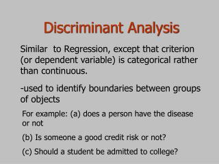
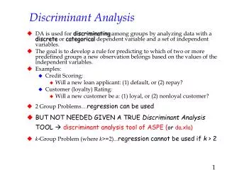
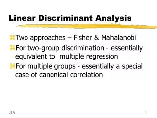
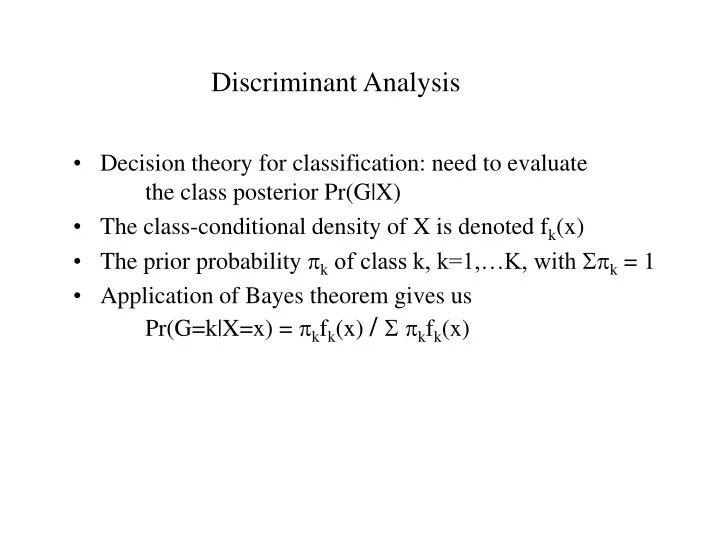
Discriminant Analysis. Decision theory for classification: need to evaluate the class posterior Pr(G|X) The class-conditional density of X is denoted f k (x) The prior probability p k of class k, k=1,…K, with p k = 1

E N D
Discriminant Analysis • Decision theory for classification: need to evaluate the class posterior Pr(G|X) • The class-conditional density of X is denoted fk(x) • The prior probability pk of class k, k=1,…K, with pk = 1 • Application of Bayes theorem gives us Pr(G=k|X=x) = pkfk(x) / pkfk(x)
Linear Discriminant Analysis • Assume fk(x) ~ Multivariate Normal(mk, S) Then, log{Pr(G=k|X=x) / Pr(G=j|X=x)} = log{fk(x) / fj(x)} + log{pk/pj} = log{pk/pj} - ½(mk+mj)TS–1(mk-mj) + xTS-1(mk-mj) > 0 xTS-1(mk-mj) > ½(mk+mj)TS–1(mk-mj) (assume pk = pj) • The LDA discriminant function is dk(x) = xTS-1mk - ½mkTS–1mk + logpk
Quadratic Discriminant Analysis • Assume fk(x) ~ Multivariate Normal(mk, Sk) Then, log{Pr(G=k|X=x) / Pr(G=j|X=x)} = log{fk(x) / fj(x)} + log{pk/pj} = (difference between log likelihoods (or densities) of N(mk, Sk) and N(mj, Sj) ) • The QDA dicriminant function dk(x) = -½ log|Sk| - ½(x-mk)TSk–1(x-mk) + logpk
Properties of LDA and QDA • Differences between LDA and QDA are small, especially if polynomial factors are considered in LDA • QDA requires to estimate each variance-covariance matrix for each class needs more observations • LDA and QDA have consistently shown high performance • Not because the data likely from Gaussian distributions • More likely because the data support only a simple boundaries such as linear or quadratic
Interpretation of tobacco parameter • Slope coefficient 0.081 with Std Error 0.026 • An increase of coronary heart disease due to tobacco factor is exp(0.081) = 1.084 or 8.4% increase • 95% confidence bound = (0.0812x0.026) =(1.03, 1.14)
Logistic Regression K-1 log-odds or logit transformations for logistic regression
LDA or Logistic Regression? • Logistic regression requires less assumption • Logistic regression maximizes the conditional likelihood Pr(G=k|X), typically by a Newton-Raphson algorithm • LDA maximizes the full log-likelihood Pr(X, G=k) = f(X; mk, S) pk (often by Least Squares estimation) • If fk(x) is Gaussian, Logistic Regression shows a loss of 30% efficiency in the (misclassification) error rate compared to LDA
Support Vector Machines (SVMs) • Support Vector Machines are a family of supervised learning algorithms for classification • Two-class classification problem: learn to predict whether a test example is positive (+1) or negative (-1)
Motivation of Support Vector Machine • Separating Hyperplanes
Binary Classification • Supervised learning: we are given labeled training set S = {(x1, y1), … , (xm, ym)} • xi are examples (e.g. protein sequences, gene expression profiles) • yi are labels: +1 or -1 • Learning algorithm selects classification rulefrom training data, S hS • Given a new test example x, trained classifier gives a prediction hS(x) (either +1 or –1)
Feature Space • SVMs require that examples are vectors • If input example are not vector valued, need a feature map into vector space: x (φ1(x),φ2(x), …, φN(x)) • Later: feature space can be defined implicitly by kernel function Training Vectors + + + + _ _ _ + _ _ _ _
Feature Maps • Sometimes, linear classifier is adequate in the original vector space • Idea: use non-linear feature map and train SVM in new feature space + + + + + _ _ + + _ + + _ _ + + + + _ + _ _ _ _ _ _ _ _ _ Input Space Feature Space _
Feature Maps • If input space is a space of discrete objects (e.g. sequences, trees), need a feature map to use SVM + ACGGTCGT CGGAAATTTA CGATTAA ACTGATAAA TTTTTAAAA ATTTTTAACAA … + + _ _ _ Input Space Feature Space
Use of Kernels • SVM dual problem and SVM classifier only use inner products <xi,xj> of training vectors • Kernel function for feature map given by: K(xi,xj) = <(xi),(xj)> • Replace <xi,xj> by K(xi,xj) in SVM solution
Some Kernels for RN • Polynomial kernels of order d K(x,y) = <x,y>d (feature space of degree = d monomials) or K(x,y) = (<x,y> + c)d (feature space of degree d monomials) • Allow fast computation in high dimensions
Example: Degree 2 Polynomial Kernel • Decision boundary induced in input space
Example: Radial Basis Kernel • K(x,y) = exp(-|x-y|2/22)
Advantages of the SVM Classifier • Minimize the risk of overfitting by choosing the maximal margin hyperplane • Obtain bounds on generalization error that depend on margin but are independent of dimension of feature space • Sparseness of classifier also leads to good generalization
Classification methods Applied to Microarray Data • Linear and quadratic discriminant analysis (LDA, QDA) • Bayesian regression model • Partial least squares method • Support vector machines (SVMs) • Logistic regression (LR) • Genetic algorithm/k-nearest neighborhood • Gene voting: For binary classification, each gene casts a vote for class 1 or 2 among p samples, and the votes are aggregated over genes A variant DLDA (diagonal LDA) • Bagging (bootstrap aggregating): perturbed learning sets by bootstrap and predictors are aggregated by community voting • Boosting … parametric distribution- free community voting
Standard Procedure for Classification Model Construction Step 1. A subset of genes that are considered most predictive for class prediction are preselected prior to modeling by e.g. two-sample t-test or SAM Step 2. Train and fit the model based on leave-one-out or n-fold cross validation on the training set Step 3. Evaluate model performance on an independent test set (External Validation; Ambroise and McLachlan, PNAS 2002)
But many questions… • Do we utilize the existing methods effectively? • Do we still need better, different kind of classification & prediction methods? • Do certain classification methods perform better on different microarray data sets? How can the best classification model(s) be chosen for a particular set, or should multiple methods be used together?
More important question • How can the subset of genes (or features) be preselected prior to modeling? And how many genes, e.g. 50, 100, or 500? Or, do we need such a large number of genes for accurate classification? • Classification accuracy depends on each data set, but neither much on the number of features in the model nor on the classification method • There must be a much smaller number of genes that can effectively discriminate the disease subtypes in different forms of their feature space
Ultimate Goals for Microarray Classification Can we identify a small number of biomarker genes with equivalent, or even better classification performance, consistently on future independent patient samples? (Robust (optimal) classification model) • These biomarker genes can then be utilized to develop a cheaper and more convenient diagnostic kit, rather than microarray profiling on each patient visit • Together with their pathway genes, they can be further investigated for their clinical relevance and treatment
Challenge 1: astronomic candidate models model dim number of all possible models from 10K array 1-gene 10,000 2-gene 49,995,000 (=4.99e+07) 3-gene 166,616,670,000 (=1.66e+11) 4-gene 416,416,712,497,500 (=4.16e+14) 5-gene 832,500,291,625,001,980 (=8.32e+17) 6-gene 1,386,806,735,798,649,200,000(=1.38e+21) …
Challenge 2: insensitive measure of classification performance • Current Measures for Classification Model Performance, such as ER (error rate) and AUC (area under ROC curve) are insensitive to the probabilistic performance differences among classification models • Example: (posterior) classification probabilities to correct classes for three samples predicted by two prediction models (two class case) model 1 model 2 Sample 1 0.60.6 Sample 2 0.90.7 Sample 3 0.30.4 ER 1/3 1/3 model 1 model 2 1.0 0.6 0.40.6 0.40.6 ER 2/3 0/3 E[Nc] 1.8 1.8 E[Nc] 1.8 1.7 E[Nc]: expected number of correctly-classified samples
New Measure of Classification Performance:Misclassification Penalized Posterior (MiPP) • More sensitive measure of classification performance, taking into account both the posterior classification probabilities and error rate pk(Xkj) = posterior classification probability of Xkjto its correct class k MiPP is the sum of the posterior probabilities of correct classification subtracted by the number of misclassified samples (NM), which varies between –N and N
Stepwise Model Construction When separate Training and Test data sets are available: Step 1: Search optimal classification models on training data by adding features sequentially and evaluating n-fold cross-validated MiPP p Initial Stage 2nd Stage G1=fk with max{p} (f1, p1) (f2, p2) Keep G1 and add remaining 9999 features to find one with maxp=G2. (f10000, p10000) kth Stage Yields optimal gene model Gk; Stop based on a stopping rule Step 2: Evaluate performance of model Gi on test set to find the most parsimonious optimal model by MiPP or ER Step 3: If feasible, use the third set for model validation
New Strategy of Classification Modeling Preselected Features Proposed Current Rule (method & criterion) Feature Selection Independent Performance Measure Validation
Examples • Two public data sets • Acute leukemia data (Golub, et al. 1999; 38 training & 34 test patient samples) • Colon cancer data (Alon et al. 1999; 40 colon patient and 22 normal samples) • Classification rules • QDA and LDA • Logistic regression • Support Vector Machines with a linear and RBF kernel
Classification Performance (MiPP) on Leukemia Test Data LDA 34 QDA Logistic SVM K=RBF SVM K=Lin 30 25 MiPP 20 15 10 1-Gene 2-Gene 3-Gene 4-Gene Gene Model
Comparison with other studies Soukup, Cho, and Lee MiPP LDA Two-Gene Robust Model = 1882 (CST3 Cystatin C (amyloid angiopathy and cerebral hemorrhage) + 1144 (SPTAN1 Spectrin, alpha, non-erythrocytic 1 (alpha-fodrin)
Classification modeling on Colon Cancer Data • Single data set • 62 samples (40 cancer samples and 22 normal samples) • 2000 of original 6500+ gene expression probes • Highest minimal intensity across 62 samples • No distinction between train and test data sets!
Split-Split Classification Modeling: Split 1. Robust Optimal Model Search Step 1: Randomly split the data with train and test sets (e.g. 2:1 ratio) Full Data Set Step 2: Create a model on the training data by sequentially adding features. Training g1= G1 g1+ g2 = G2 g1+g2+…+gk = Gk Using MiPP Step 3: Evaluate each model on the test data set based on MiPP Test MiPP or ER Repeat Step 1-3 B (e.g. 20) times