Download
1 / 66
660 likes | 676 Views
Learn about vector and matrix norms, condition number, ill-conditioning, basic iterative methods, and their applications in numerical solutions of linear systems. Understand how to assess the sensitivity of a system to errors and data perturbations.

E N D
CSE 551 Computational Methods 2018/2019 Fall Chapter 7-B Iterative Solutions of Linear Systems
Outline Vector and Matrix Norms Condition Number and Ill-Conditioning Basic Iterative Methods Pseudocode Convergence Theorems Matrix Formulation Another View of Overrelaxation Conjugate Gradient Method
References • W. Cheney, D Kincaid, Numerical Mathematics and Computing, 6ed, • Chapter 8
Iterative Solutions of Linear Systems • a completely different strategy for solving a nonsingular linear system • used • solving partial differential equations numerically. • systems having hundreds of thousands of equations arise routinely
Vector and Matrix Norms • useful in the discussion of errors and in the stopping criteria for iterative methods • defined on any vector space, • Rnor Cn • A vector norm ||x|| - length or magnitude of a vector x Rn • any mapping from Rnto R • properties: for vectors x, y Rnand scalars α R
Examples of vector norms • for vector x (x1, x2, . . . , xn)T Rn:
n × n matrices, - matrix norms, subject to the same requirements: • for matrices A, B and scalars α.
matrix norms that are related to a vector norm. • For a vector norm || · ||, the subordinate matrix norm is defined by • A n × n matrix • subordinate matrix norm - additional properties:
two meanings - with the notation || · ||p • vectors, matrices • The context will determine which one is intended. Examples of subordinate matrix norms • for an n × n matrix A: • σi: eigenvalues of ATA - singular values of A • largest σmax in absolute value spectral radius of A
Condition Number and Ill-Conditioning • important quantity influence in the numerical solution of a linear system • Ax = b - the condition number, defined: • not necessary to compute the inverse of A obtain an estimate of the condition number
the condition number κ(A) gauges the • transfer of error from the matrix A and the vector b to the solution x • The rule of thumb: • if κ(A) = 10k, expect to lose at least k digits of precision in solving the system Ax = b • If the linear system is sensitive to perturbations in • elements of A, components of b • reflected in A having a large • condition number • In such a case, the matrix A is said to be ill-conditioned. • the larger the condition number, the more ill-conditioned the system.
to solve an invertible linear system of equations Ax = b for a given coefficient matrix A and right-hand side b • there may have been perturbations of the data • owing to uncertainty in the measurements • and roundoff errors in the calculations. • Suppose that • right-hand side is perturbed by an amount δb • corresponding solution is perturbed an amount δx.
From the original linear system Ax = b and norms, • From the perturbed linear system Aδx = δb, • δx = A−1δb
Combining the two inequalities: • contains the condition number of the original matrix A.
example of an ill-conditioned matrix - the Hilbert matrix: • condition number: 524.0568 • determinant: 4.6296×10⁻⁴ • In solving linear systems, • the condition number of the coefficient matrix measures the sensitivity of the system to errors in the data
When the condition number large • the computed solution of the system • may be dangerously in error! • Further checks should be made before accepting the solution • as being accurate • Values of the condition number near 1 indicate a well-conditioned matrix • whereas large values indicate an ill-conditioned matrix. Using the determinant to check for • singularity is appropriate only for matrices of modest size. • Using mathematical software, • compute the condition number to check for singular or near-singular matrices.
A goal in the study of numerical methods is to acquire an awareness of • whether a numerical result can be trusted or • whether it may be suspect (and therefore in need of further analysis). • condition number - some evidence regarding this question. • In fact, some solution procedures involve • advanced features that depend on an estimated condition number and may switch solution • techniques based on it.
For example, this criterion may result in a switch of the solution technique from a variant of Gaussian elimination to a least-squares solution for an illconditioned system. • Unsuspecting users may not realize that this has happened unless they look at all of the results, including the estimate of the condition number. • (Condition numbers • can also be associated with other numerical problems, such as locating roots of equations.)
Basic Iterative Methods • produces sequence of approximate solution vectors x(0),x(1), x(2), . . . for system Ax = b • designed - the sequence converges to the actual solution. • stopped - sufficient precision attained • contrast to Gaussian elimination algorithm, • no provision for stopping midway • and offering up an approximate solution
general iterative algorithm for solving System (1) : • Select • a nonsingular matrix Q • and having chosen an arbitrary starting vector x(0) • generate vectors • x(1), x(2), . . . recursively: • suppose that the sequence x(k)does converge, to a vector x*, taking the limit as k →∞in System (2):
leads to Ax* = b • if the sequence converges, • its limit - solution to System (1) • e.g., Richardson iteration uses Q = I.
In choosing - nonsingular matrix Q : • System (2) - easy to solve for x(k), when the right-hand side is known. • Matrix Q should be chosen to ensure that the sequence x(k)converges, no matter what initial vector is used. • Ideally, this convergence will be rapid. • not necessary to compute the inverse of Q • solve a linear system - Q:coefficient matrix. • select Q - easy to solve • e.g., diagonal, tridiagonal, banded, lower triangular, and upper triangular.
System (1) in detailed form: • Solving the ith equation for the ith unknown term, Jacobi method: • assume that all diagonal elements are nonzero • If not rearrange the equations
In the Jacobi method,the equations are solved in order • xj(k−1)and • Gauss-Seidel method: • new values xj(k−1) can be used immediately in their place.
acceleration of the Gauss-Seidel method • relaxation factor ω - successive overrelaxation (SOR) method: • SOR method with ω = 1 reduces to the Gauss-Seidel method.
Example • (Jacobi iteration) Let • Carry out a number of iterations of the Jacobi iteration, starting with the zero initial vector.
Example • Rewriting the equations, Jacobi method: • initial vector x(0)= [0, 0, 0]T • The actual solution (to four decimal places rounded) obtained
Jacobi iterative matrix and constant vector: • Q close to A, Q−1A close to I, I − Q−1A small. the
Example • (Gauss-Seidel iteration) Repeat the preceding example using the Gauss-Seidel iteration. • Solution • The idea of the Gauss-Seidel iteration: • accelerate the convergence - incorporating each vector as soon as it has been computed • more efficient in the Jacobi method to use the updated value x1(k) in the second equation instead of the old • value x1(k-1) • Similarly, x2(k) could be used in the third equation in place of x2(k-1)
Using the new iterates as soon as they become available, Gauss-Seidel method: • Starting with the initial vector zero, some of the iterates:
In this example, the convergence of the Gauss-Seidel method is approximately twice as fast • as that of the Jacobi method • In Gauss-Seidel, Q – lower triangular part of A, including the diagonal. • Using the data from the previous example:
in a practical problem not compute Q−1. • Gauss- Seidel iterative matrix and constant vector • Gauss-Seidel method:
Example • (SOR iteration) Repeat the preceding example using the SOR iteration with ω = 1.1. • Starting with the initial vector – zeros, with ω = 1.1, some of the iterates:
the convergence of the SOR method is faster than that of the Gauss-Seidel method • SOR - Q - lower triangular part of A including the diagonal, but each diagonal element • ai j replaced by ai j/ω, ω relaxation factor.
SOR iterative matrix and constant vector: • write the SOR method:
the vector y contains the old iterate values, • and the vector x contains the updated ones • The values of kmax, δ, and ε are set either in a parameter statement or as global variables.
The pseudocode for the procedure Gauss Seidel(A, b, x) would be the same as that for the Jacobi pseudocode above except that the innermost j-loop would be replaced by the following:
The pseudocode for procedure SOR(A, b, x, ω)would be the same as that for the Gauss- • Seidel pseudocode with the statement following the j-loop replaced by: xi ← sum/diag xi ← ωxi + (1 − ω)yi • In the solution of partial differ
Convergence Theorems • For the analysis of the method described by System (2): • the iteration matrix and vector:
in the pseudocode, not compute Q−1 • to facilitate the analysis • et x be the solution of System (1) • Since A nonsingular, x exists and is unique • from Equation (7), • e(k)≡ x(k)− x current error vector
e(k)to become smaller as k increases • Equation (8) - e(k)will be smaller than e(k-1) • if I − Q−1A is small, in some sense • Q−1A close to I. • Q should be close to A. • (Norms can be used to make small and close • precise.)
THEOREM 1 SPECTRAL RADIUS THEOREM • In order that the sequence generated by • Qx(k)= (Q − A)x(k-1)+ b to converge, • no matter what starting point x(0)is selected • it is necessary and sufficient that all • eigenvalues of I − Q−1A lie in the open unit disc, |z| < 1, in the complex plane.
The conclusion of this theorem can also be written as • where ρ is the spectral radius function: For any n × n matrix G, having eigenvalues • λi, ρ(G) = max1in|λi |.
Example • Determine whether the Jacobi, Gauss-Seidel, and SOR methods (with ω = 1.1) of the • previous examples converge for all initial iterates. • Solution
the Jacobi method, compute the eigenvalues of the relevant matrix B. • The steps are • The eigenvalues are λ = 0,±sqrt(1/3) ≈ ±0.5774 • by the preceding theorem: • Jacobi iteration succeeds for any starting vector in this example.