Download
1 / 42
420 likes | 567 Views
Trace polynomial for homotopy classes of simple closed curves on the twice punctured torus. Raquel Águeda Maté UCLM (Spain). L. Bers (60’s): Transition from discrete to non-discrete groups?. D. Mumford and D. Wright (80’s): First computer explorations. L. Keen and C. Series (late 80’s).

E N D
Trace polynomial for homotopy classes of simple closed curves on the twice punctured torus Raquel Águeda Maté UCLM (Spain)
L. Bers (60’s): Transition from discrete to non-discrete groups? D. Mumford and D. Wright (80’s): First computer explorations. L. Keen and C. Series (late 80’s) Introduction
D. Mumford, C. Series and D. Wright, Indra’s Pearls, CUP (2002)
Deformation space of free Kleinian groups Γ. Γ Kleinian group: discrete subgroup of PSL(2, ). Γ generated by two elements: parabolic and loxodromic (trace ±2 and complex resp.). Introduction
Discrete, faithful and type-preserving representations of the fundamental group of a hyperbolic 3-manifold M in PSL(2, ) : ρ: π1(M) PSL(2, ) M is obtained by pinching a non-dividing curve in a handlebody of genus 2. Introduction
3 Introduction
Γ acts properly discontinuously on (Γ discrete group). The action of Γ divides on: 1. Λ(Γ) = limit set, 2. Ω(Γ) = \ Λ(Γ) = regular set. Γ acts properly discontinuously on Ω(Γ). Mp ( 3 ()) / H Introduction
The convex hull (Γ) of the limit set is the closure of the set geodesics that join each pair of points of Λ(Γ) in . (Γ) / Γ istheconvex core: the smallest convex set that contains all the geodesics in / Γ. The boundary of (Γ) is a pleated surface: pieces of hyperbolic planes that meet along a geodesic lamination. Pleating locus invariant by Γ. Invariant of the metric in . ( (Γ)/ Γ) is homeomorphic to M . Introduction
Introduction (Γ) C Ax(g)
Introduction Y. Y. Minsky Minsky (en (en Indra’s Pearls Indra’s Pearls ) )
Introduction Y. Y. Minsky Minsky (en (en Indra’s Pearls Indra’s Pearls ) )
Pleating variety, : locus in where is pleated along . is the locus where the curves in have real trace (Y. Choi and C. Series). (C()/Γ) can be calculated by studying pleating varieties. : some curve in becomes parabolic. Introduction (X,Y ) : ((X,Y) ) / (X,Y) 2 C = R is a twice punctured torus
4 4 Introduction
1 Introduction
Analysis Discrete and faithful representations ρ: π1(M) PSL(2, ) Geometry Combinatorics Curve systems in M Introduction o Geometric structures in M Measured laminations: bending locus of the convex core boundary of M.
Aim Find the parameter space and its boundary . R / R Idea Introduction Use pleating variaties.
Definition A curve system in Mis a family of disjoint essential simple loops whose components are homotopically distinct. Homotopy classes of curve systems
Parametrization of ∂M-homotopy classes of curve systems [Keen - Parker - Series] 2 1 1 Homotopy classes of curve systems
Normalize the set of generators of Γρ. Homotopy classes of curve systems Set up a set of generators for Γρ. B = oi* (1), A = oi* (1), Id = oi*(2)
B A-1 A 2 2 1 3 2 2 C-1 C 1 1 2 2 1 B-1 1 1 2 2 Homotopy classes of curve systems Example ρ ( γ1 ) = BA-1BC-1AB-1B-1C ρ ( γ2 ) = BC-1
yi xi yi xi ui ui yi yi xi xi Homotopy classes of curve systems
1 2 2 3 2 2 2 1 Homotopy classes of curve systems p ( ) = ( 5, 3, 2, 1 )
We find in every M-homotopy class a representative curve system in M, unique up to ∂M-homotopy, such that q1 ( ) ≤ q2 ( ) and 0 ≤ p2 ( ) ≤ q2 ( ). Homotopy classes of curve systems When are homotopic in M two curve systems which are non-homotopic in ∂M ?
: homeomorphisms of that extend to M and are homotopic to the identity. 1. Extensions of Dehn twists along compressible curves. 2. Hyperelliptic involution. Homotopy classes of curve systems
1. Extensions of Dehn twists around compressible curves: α2, δ and ταn (δ), n Homotopy classes of curve systems 2 1
1 2 Homotopy classes of curve systems 2. Hyperelliptic involution f. 2 1
THEOREM Homotopy classes of curve systems
Proposition Let a curve system in M and g a homeomorphism of M, then q2 ( g ( )) = q2 ( ). Reducing process: q1 ( g ( )) < q1 ( ), while q2 ( g ( )) = q2 ( ). Homotopy classes of curve systems
Proposition If q2 < q1, p1 > 0 and p1 < q1, then: Homotopy classes of curve systems
Homotopy classes of curve systems Corollary
¿What if q1 does not get reduced by using τδ? Homotopy classes of curve systems Proposition
æ g is: Homotopy classes of curve systems Proposition
Homotopy classes of curve systems Proposition
We compute the first two terms of the trace polynomial of curves in the canonic form in terms of their p-coordinates. Trace polynomial Which is the trace polynomial?
THEOREM Let γ be a simple closed curve on M with p-coordinates p(γ) = ( q1, q2, p1, p2 )where q1 ≤ q2 ≠ 0 and 0 ≤ p2 < q2. Let ρ(γ) the image of the curve γ by the representation ρ in PSL(2, ). Then the top term of the trace polynomial of ρ(γ) is a homogeneous polynomial of degree q2 on the complex variables X and Y with the following form: Furthermore, the term of degree q2 1 vanishes. Trace polynomial
Proof Trace polynomial By induction on
In the conditions of last theorem: Trace polynomial Corollary
Trace polynomial for homotopy classes of simple closed curves on the twice punctured torus Raquel Águeda Maté UCLM (Spain)