Analysis of Variance (ANOVA)

1. Analysis of Variance (ANOVA)

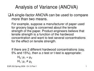
2. Analysis of Variance (ANOVA) • Hypothesis H0 : mi = mG H1:  i | (mi  mG ) • Logic S2within = error variability S2between = error variability + treatment Where, x = grand mean, xj = group mean, k = number of groups, nj = number of participants in a group, N = Total number of participants

3. Classic ANOVA Table Total variability = Between variability + within variability Sums of square

4. Computation Degrees of freedom Means square F

5. ANOVA

6. Analysis of Variance (ANOVA) • If the independent variables are continuous and the dependant variable is also continuous then we will perform a multiple regression. Now, if the independent variables are discrete and the dependant variable is still continuous we will performed an ANOVA where, m = grand mean, t = treatment effect, e = error From ANOVA To GLM where,

7. Analysis of Variance (ANOVA) • Example

8. Analysis of Variance (ANOVA) Using the GLM approach through a coding matrix • Logic: • If, for example, there are 3 groups and we know that the participant number 12 is not part of the first nor the second group, then we know that this participant is necessary part of group 3.

9. Analysis of Variance (ANOVA) Performing ANOVA using GLM through a coding matrix • Logic: • In other words, there is only 2 degrees of freedom in group assignation. Therefore, the third group column will be eliminated. • A value of 1 will be assigned to the participants of group i and a value of 0 for the other groups. Whereas, the last group will receive a value of -1 for all the group (balance things).

10. Analysis of Variance (ANOVA) Then, for each subject we associate its corresponding group coding. = independent variables (X)

11. Analysis of Variance (ANOVA) X y A = SSCP =

12. R-Square • R2 is obtained by: SSCP = Number of participants Number of predictors (independent variables)

13. ANOVA Table • The hypothesis is that the R-Square between the predictors and the criterion is null. Since F(3,32)=5.86938, p<0.05, we reject H0 and we accept H1. There is at least one group that is different from the others.

14. ANOVA Terminology • Coefficient of determination (proportion of explained variation)

15. ANOVA • Now you know it! • ANOVA is a special case of regression. • The same logic can be applied to t-test, factorial ANOVA, ANCOVA, simple effects (Tukey, Bonferoni, LSD, etc.)

16. Principal Component Analysis (PCA)

17. PCA • Why • To discover or to reduce the dimensionality of the data set. • To identify new meaningful underlying variables • Assumptions • Sample size : about 300 (in general) • Normality • Linearity • Absence of outliers among cases

18. PCA • Illustration Second principal component First principal component

19. PCA • Preliminary • Data • Z scores X = Zx=

20. PCA • Preliminary • SSCP • Correlation Matrix SSCP = M =

21. PCA • Eigenvalues and eigenvectors • Let’s define a random vector as v(0) = [1, 1]T. Now, if we compute the inner product between the correlation matrix (M) and V(0) an re-multiply the result by M, again, again, and again, what the results will be after k iterations?

22. PCA • Eigenvalues and eigenvectors • Let’s define a random vector as v(0) = [1, 1]T. Now, if we compute the inner product between the correlation matrix (M) and V(0) an re-multiply the result by M, again, again, and again, what the results will be after k iterations?

23. PCA • Eigenvalues and eigenvectors • After convergence • 1- The direction of the stable vector = Eigenvector () • 2- The stable vector lengthening factor = Eigenvalue ()

24. PCA • Eigenvalues and eigenvectors • Once the first eigenvector (and associated eigenvalue) has been identified, we remove it from the matrix. • And we repeat the process until all the eigenvectors and eigenvalues have been extracted.

25. PCA • Eigenvalues and eigenvectors • There will be as many eigenvectors/eigenvalues as there are variables. • Each eigenvector will be orthogonal to the others. M = PCA

26. PCA • Eigenvalues and eigenvectors • There will be as many eigenvectors/eigenvalues as there are variables. • Each eigenvector will be orthogonal to the others. 1 2 3 4

27. PCA • Eigenvalues and eigenvectors • How many are important? Plot the eigenvalues, • 1- If the points on the graph tend to level out (show an "elbow"), these eigenvalues are usually close enough to zero that they can be ignored. • 2- Limit variance accounted for, (e.g. 90%) Method 1 Method 2

28. PCA • Eigenvalues and eigenvectors • Illustration of the data and the selected eigenvectors = FT 2 x3 x1 x2 x4 1

29. PCA • VARIMAX Rotation • Why ? To improve the readability • The VARIMAX rotation aims at finding a solution where an original variable loads highly on one particular factor and loads as low as possible on other factors.  Rotation matrix

30. (X-X)2 PCA • VARIMAX Rotation • The algorithm maximizes the VARIMAX index, V, the sum of the variances of the component-loading matrix. • V will be a long equation that contains the q variable. An optimization technique is then used to find the value q that maximize V.

31. PCA • VARIMAX Rotation • The algorithm maximizes the VARIMAX index, V, the sum of the variances of the component-loading matrix. U = V =

32. PCA • VARIMAX Rotation • The algorithm maximizes the VARIMAX index, V, the sum of the variances of the component-loading matrix. 2 2 x3 x3 1 x1 x2 x2 x1 x4 1 x4