Download
1 / 33
330 likes | 437 Views
Chapter 6: CPU Scheduling. Basic Concepts Scheduling Criteria Scheduling Algorithms Multiple-Processor Scheduling Real-Time Scheduling Algorithm Evaluation. Basic Concepts. Maximum CPU utilization obtained with multiprogramming

E N D
Chapter 6: CPU Scheduling • Basic Concepts • Scheduling Criteria • Scheduling Algorithms • Multiple-Processor Scheduling • Real-Time Scheduling • Algorithm Evaluation 111/19/2014
Basic Concepts • Maximum CPU utilization obtained with multiprogramming • CPU–I/O Burst Cycle – Process execution consists of a cycle of CPU execution and I/O wait. • CPU burst distribution 211/19/2014
Alternating Sequence of CPU And I/O Bursts 311/19/2014
Histogram of CPU-burst Times 411/19/2014
CPU Scheduler • Selects from among the processes in memory that are ready to execute, and allocates the CPU to one of them. • CPU scheduling decisions may take place when a process: 1. Switches from running to waiting state. 2. Switches from running to ready state. 3. Switches from waiting to ready. 4. Terminates. • Scheduling under 1 and 4 is nonpreemptive. • All other scheduling is preemptive. 511/19/2014
Dispatcher • Dispatcher module gives control of the CPU to the process selected by the short-term scheduler; this involves: • switching context • switching to user mode • jumping to the proper location in the user program to restart that program • Dispatch latency– time it takes for the dispatcher to stop one process and start another running. 611/19/2014
Scheduling Criteria • CPU utilization – keep the CPU as busy as possible • Throughput – # of processes that complete their execution per time unit • Turnaround time – amount of time to execute a particular process • Waiting time – amount of time a process has been waiting in the ready queue • Response time – amount of time it takes from when a request was submitted until the first response is produced, not output (for time-sharing environment) 711/19/2014
Optimization Criteria • Max CPU utilization • Max throughput • Min turnaround time • Min waiting time • Min response time 811/19/2014
P1 P2 P3 0 24 27 30 First-Come, First-Served (FCFS) Scheduling ProcessBurst Time P1 24 P2 3 P3 3 • Suppose that the processes arrive in the order: P1 , P2 , P3 The Gantt Chart for the schedule is: • Waiting time for P1 = 0; P2 = 24; P3 = 27 • Average waiting time: (0 + 24 + 27)/3 = 17 911/19/2014
P2 P3 P1 0 3 6 30 FCFS Scheduling (Cont.) Suppose that the processes arrive in the order P2 , P3 , P1 . • The Gantt chart for the schedule is: • Waiting time for P1 = 6;P2 = 0; P3 = 3 • Average waiting time: (6 + 0 + 3)/3 = 3 • Much better than previous case. • Convoy effect short process behind long process 1011/19/2014
Shortest-Job-First (SJR) Scheduling • Associate with each process the length of its next CPU burst. Use these lengths to schedule the process with the shortest time. • Two schemes: • nonpreemptive – once CPU given to the process it cannot be preempted until completes its CPU burst. • preemptive – if a new process arrives with CPU burst length less than remaining time of current executing process, preempt. This scheme is know as the Shortest-Remaining-Time-First (SRTF). • SJF is optimal – gives minimum average waiting time for a given set of processes. 1111/19/2014
P1 P3 P2 P4 0 3 7 8 12 16 Example of Non-Preemptive SJF Process Arrival TimeBurst Time P1 0.0 7 P2 2.0 4 P3 4.0 1 P4 5.0 4 • SJF (non-preemptive) • Average waiting time = (0 + 6 + 3 + 7)/4 - 4 1211/19/2014
P1 P2 P3 P2 P4 P1 11 16 0 2 4 5 7 Example of Preemptive SJF Process Arrival TimeBurst Time P1 0.0 7 P2 2.0 4 P3 4.0 1 P4 5.0 4 • SJF (preemptive) • Average waiting time = (9 + 1 + 0 +2)/4 - 3 1311/19/2014
Determining Length of Next CPU Burst • Can only estimate the length. • Can be done by using the length of previous CPU bursts, using exponential averaging. 1411/19/2014
Prediction of the Length of the Next CPU Burst 1511/19/2014
Examples of Exponential Averaging • =0 • n+1 = n • Recent history does not count. • =1 • n+1 = tn • Only the actual last CPU burst counts. • If we expand the formula, we get: n+1 = tn+(1 - ) tn -1 + … +(1 - )j tn -1 + … +(1 - )n=1 tn 0 • Since both and (1 - ) are less than or equal to 1, each successive term has less weight than its predecessor. 1611/19/2014
Priority Scheduling • A priority number (integer) is associated with each process • The CPU is allocated to the process with the highest priority (smallest integer highest priority). • Preemptive • nonpreemptive • SJF is a priority scheduling where priority is the predicted next CPU burst time. • Problem Starvation – low priority processes may never execute. • Solution Aging – as time progresses increase the priority of the process. 1711/19/2014
Round Robin (RR) • Each process gets a small unit of CPU time (time quantum), usually 10-100 milliseconds. After this time has elapsed, the process is preempted and added to the end of the ready queue. • If there are n processes in the ready queue and the time quantum is q, then each process gets 1/n of the CPU time in chunks of at most q time units at once. No process waits more than (n-1)q time units. • Performance • q large FIFO • q small q must be large with respect to context switch, otherwise overhead is too high. 1811/19/2014
P1 P2 P3 P4 P1 P3 P4 P1 P3 P3 0 20 37 57 77 97 117 121 134 154 162 Example of RR with Time Quantum = 20 ProcessBurst Time P1 53 P2 17 P3 68 P4 24 • The Gantt chart is: • Typically, higher average turnaround than SJF, but better response. 1911/19/2014
Time Quantum and Context Switch Time 2011/19/2014
Turnaround Time Varies With The Time Quantum 2111/19/2014
Multilevel Queue • Ready queue is partitioned into separate queues:foreground (interactive)background (batch) • Each queue has its own scheduling algorithm, foreground – RRbackground – FCFS • Scheduling must be done between the queues. • Fixed priority scheduling; (i.e., serve all from foreground then from background). Possibility of starvation. • Time slice – each queue gets a certain amount of CPU time which it can schedule amongst its processes; i.e., 80% to foreground in RR • 20% to background in FCFS 2211/19/2014
Multilevel Queue Scheduling 2311/19/2014
Multilevel Feedback Queue • A process can move between the various queues; aging can be implemented this way. • Multilevel-feedback-queue scheduler defined by the following parameters: • number of queues • scheduling algorithms for each queue • method used to determine when to upgrade a process • method used to determine when to demote a process • method used to determine which queue a process will enter when that process needs service 2411/19/2014
Example of Multilevel Feedback Queue • Three queues: • Q0– time quantum 8 milliseconds • Q1– time quantum 16 milliseconds • Q2– FCFS • Scheduling • A new job enters queue Q0which is servedFCFS. When it gains CPU, job receives 8 milliseconds. If it does not finish in 8 milliseconds, job is moved to queue Q1. • At Q1 job is again served FCFS and receives 16 additional milliseconds. If it still does not complete, it is preempted and moved to queue Q2. 2511/19/2014
Multilevel Feedback Queues 2611/19/2014
Multiple-Processor Scheduling • CPU scheduling more complex when multiple CPUs are available. • Homogeneous processors within a multiprocessor. • Load sharing • Asymmetric multiprocessing– only one processor accesses the system data structures, alleviating the need for data sharing. 2711/19/2014
Real-Time Scheduling • Hard real-time systems – required to complete a critical task within a guaranteed amount of time. • Soft real-time computing – requires that critical processes receive priority over less fortunate ones. 2811/19/2014
Dispatch Latency 2911/19/2014
Algorithm Evaluation • Deterministic modeling – takes a particular predetermined workload and defines the performance of each algorithm for that workload. • Queueing models • Implementation 3011/19/2014
Evaluation of CPU Schedulers by Simulation 3111/19/2014
Solaris 2 Scheduling 3211/19/2014
Windows 2000 Priorities 3311/19/2014