Download
1 / 53
530 likes | 674 Views
MPI-izing Your Program. CSCI 317 Mike Heroux. Simple Example. Example : Find the max of n positive numbers. Way 1: Single processor ( SISD - for comparison). Way 2: Multiple processor, single memory space (SPMD/SMP). Way 3: Multiple processor, multiple memory spaces. (SPMD/DMP).

E N D
MPI-izing Your Program CSCI 317 Mike Heroux CSCI 317 Mike Heroux
Simple Example • Example: Find the max of n positive numbers. • Way 1: Single processor ( SISD - for comparison). • Way 2: Multiple processor, single memory space (SPMD/SMP). • Way 3: Multiple processor, multiple memory spaces. (SPMD/DMP).
SISD Case maxval= 0; /* Initialize */ for (i=0; i < n; i++) maxval= max(maxval,val(i)); Processor Memory val[0] … val[n-1]
SPMD/SMP Case Processors maxval = 0; #pragma omp parallel default(none) \ shared(maxval) { intlocalmax = 0; #pragma omp for for (inti=0; i< n; ++i) { localmax = (val[i]>localmax) ? val[i]: localmax; } #pragma omp critical { maxval= (maxval>localmax) ? maxval:localmax; } } 0 Memory 1 val[0…n-1] 2 3
SPMD/DMP Case (np=4, n=16) Processors Memory Network maxval= 0; localmax = 0; for (i=0; i < 4; i++) localmax= (localmax>val[i]) ? localmax: val[i]; MPI_Allreduce(&localmax, &maxval, 1, MPI_INT, MPI_MAX, MPI_COMM_WORLD); 0 val[0…3] p = 0 1 val[0…3] = val[4…7] p = 1 val[0…3] = val[8…11] 2 p = 2 val[0…3] = val[12…15] 3 p = 3
Shared Memory Model Overview • All Processes share the same memory image. • Parallelism often achieved by having processors take iterations of a for-loop that can be executed in parallel. • OpenMP, Intel TBB.
Message Passing Overview • SPMD/DMP programming requires “message passing”. • Traditional Two-sided Message Passing • Node p sends a message. • Node q receives it. • p and q are both involved in transfer of data. • Data sent/received by calling library routines. • One-sided Message Passing (mentioned only here) • Node p puts data into the memory of node q. or • Node p gets data from the memory of node q. • Node q is not involved in transfer. • Put’ing and Get’ing done by library calls.
MPI - Message Passing Interface • The most commonly used message passing standard. • The focus of intense optimization by computer system vendors. • MPI-2 includes I/O support and one-sided message passing. • The vast majority of today’s scalable applications run on top of MPI. • Supports derived data types and communicators.
Hybrid DMP/SMP Models • Many applications exhibit a coarse grain parallel structure and a simultaneous fine grain parallel structure nested within the coarse. • Many parallel computers are essentially clusters of SMP nodes. • SMP parallelism is possible within a node. • DMP is required across nodes. • Compels us to consider programming models where, for example, MPI runs across nodes and OpenMP runs within nodes.
First MPI Program • Simple program to measure: • Asymptotic bandwidth (send big messages). • Latency (send zero-length messages). • Works with exactly two processors. CSCI 317 Mike Heroux
SimpleCommTest.cpp • Go to SimpleCommTest.cpp • Download on Linux system. • Setup: • module avail (locate MPI environment, GCC or Intel). • module load … • Compile/run: • mpicxxSimpleCommTest.cpp • mpirun -np 2 a.out • Try: mpirun -np 4 a.out • Why does it fail? How? CSCI 317 Mike Heroux
Going from Serial to MPI • One of the most difficult aspects of DMP is: There is no incremental way to parallelize your existing full-featured code. • Either a code run in DMP mode or it doesn’t. • One way to address this problem is to: • Start with a stripped down version of your code. • Parallelize it and incrementally introduce features into the code. • We will take this approach.
Parallelizing CG • To have a parallel CG solver we need to: • Introduce MPI_Init/MPI_Finalize into main.cc • Provide parallel implementations of: • waxpby.cpp, compute_residual.cpp, ddot.cpp(easy) • HPCCG.cpp(also easy) • HPC_sparsemv.cpp(hard). • Approach: • Do the easy stuff. • Replace (temporarily) the hard stuff with easy.
Parallelizing waxpby • How do we parallelize waxpby? • Easy: You are already done!!
Parallelizing ddot • Parallelizing ddot is very straight-forward given MPI: // Reduce what you own on a processor. ddot(my_nrow, x, y, &my_result); //Use MPI's reduce function to collect all partial sums MPI_Allreduce(&my_result, &result, 1, MPI_DOUBLE, MPI_SUM, MPI_COMM_WORLD); • Note: • Similar works for compute_residual. • Replace MPI_SUM with MPI_MAX. • Note: There is a bug in the current version!
Overview • Distributed sparse MV is the most challenging kernel of parallel CG. • Communication determined by: • Sparsity pattern. • Distribution of equations. • Thus, communication pattern must be determined dynamically, i.e., at run-time.
Goals • Computation should be local. • We want to use our best serial (or SMP) Sparse MV kernels. • Must transform the matrices to make things look local. • Speed (obvious). How: • Keep a balance of work across processors. • Minimize the number of off-processor elements needed by each processor. • Note: This goes back to the basic questions: “Who owns the work, who owns the data?”.
Example w A x w1 11 12 0 14 x1 w2 21 22 0 24 x2 = * w3 0 0 33 34 x3 w4 41 42 43 24 x4 Need to: • Transform A on each processor (localize). • Need to communicate x4 from PE 1 to 0. • Need to communicate x1, x2 from PE 0 to 1. - On PE 0 - On PE 1
On PE 0 w A x w1 11 12 14 x1 w2 21 22 24 x2 = * x3 x4 Note: • A is now 2x3. • Prior to calling sparse MV, must get x4. • Special note: Global variable x4 is: • x2 on PE 1. • x3 on PE 0. - On PE 0 - On PE 1 - Copy of PE 1on PE 0
On PE 1 w A x w3 33 34 0 0 x1 w4 43 24 41 42 x2 = * x3 x1 Note: • A is now 2x4. • Prior to calling sparse MV, must get x1, x2. • Special note: Global variables get remapped. x3 x1 x4 x2 x1 x3 x2 x4 x4 x2 - On PE 0 - On PE 1 - Copy of PE 0 on PE 1
To Compute w = Ax • Once the global matrix is transformed, computing Sparse_MV is: • Step one: Copy needed elements of x. • Send x4 from PE 1 to PE 0. • NOTE: x4 is stored as x2 on PE 1 and will be in x3 on PE 0! • Send x1 and x2 from PE 0 to PE 1. • NOTE: They will be stored as x3 and x4, resp. on PE 1! • Call sparsemv to compute w. • PE 0 will compute w1 and w2. • PE 1 will compute w3 and w4. • NOTE: The call of sparsemv on each processor has no knowledge that it is running in parallel!
Observations • This approach to computing sparse MV keeps all computation local. • Achieves first goal. • Still need to look at: • Balancing work. • Minimizing communication (minimize # of transfers of x entries).
HPCCG with MPI • Edit Makefile: • Uncomment USE_MPI = -DUSING_MPI • Switch to CXX and LINKER = mpicxx • DON’T uncomment MPI_INC (mpicxx handles this). • To run: • module avail (locate MPI environment, GCC or Intel). • module load … • mpirun -np 4 test_HPCCG 100 100 100 • Will run on four processors with 100-cubed local problem • Global size is 100 by 100 by 400. CSCI 317 Mike Heroux
Computational Complexity of Sparse_MV for (i=0; i< nrow; i++) { double sum = 0.0; const double * constcur_vals = ptr_to_vals_in_row[i]; constint * constcur_inds = ptr_to_inds_in_row[i]; constintcur_nnz = nnz_in_row[i]; for (j=0; j< cur_nnz; j++) sum += cur_vals[j]*x[cur_inds[j]]; y[i] = sum; } How many adds/multiplies? CSCI 317 Mike Heroux
Balancing Work • The complexity of sparse MV is 2*nz. • nz is number of nonzero terms. • We have nz adds, nz multiplies. • To balance the work we should have the same nz on each processor. • Note: • There are other factors such as cache hits that affect the sparse MV performance. • Addressing these is an area of research. CSCI 317 Mike Heroux
Example: y = AxPattern of A (X=nonzero) CSCI 317 Mike Heroux
Example 2: y = AxPattern of A (X=nonzero) CSCI 317 Mike Heroux
Example 3: y = AxPattern of A (X=nonzero) CSCI 317 Mike Heroux
Matrices and Graphs • There is a close connection between sparse matrices and graphs. • A graph is defined to be • A set of vertices • With a corresponding set of edges. • An edge exist if there is a connection between two vertices. • Example: • Electric Power Grid. • Substations are vertices. • Power lines are edges. CSCI 317 Mike Heroux
The Graph of a Matrix • Let the equations of a matrix be considered as vertices. • An edge exists between two vertices j and k if there is a nonzero value ajkor akj. • Let’s see an example... CSCI 317 Mike Heroux
6x6 Matrix and Graph a110 0 0 0 a16 0 a22a23 0 0 0 A = 0 a32a33 a34 a35 0 0 0 a43 a44 0 0 0 0 a53 0 a55a56 a61 0 0 0 a65a66 2 1 3 6 4 5 CSCI 317 Mike Heroux
“Tapir” Matrix (John Gilbert) CSCI 317 Mike Heroux
Corresponding Graph CSCI 317 Mike Heroux
2-wayPartitioned Matrix and Graph a110 0 0 0 a16 0 a22a23 0 0 0 A = 0 a32a33 a43 a35 0 0 0 a43 a44 0 0 0 0 a53 0 a55a56 a61 0 0 0 a65a66 2 1 3 6 4 5 • Questions: • How many elements must go from PE 0 to 1 and 1 to 0? • Can we reduce this number? Yes! Try: 2 1 3 6 4 5 CSCI 317 Mike Heroux
3-wayPartitioned Matrix and Graph a110 0 0 0 a16 0 a22a23 0 0 0 A = 0 a32a33 a43 a35 0 0 0 a43 a44 0 0 0 0 a53 0 a55a56 a61 0 0 0 a65a66 2 1 3 6 4 5 • Questions: • How many elements must go from PE 1 to 0, 2 to 0, 0 to 1, 2 to 1, 0 to 2 and 1 to 2? • Can we reduce these number? Yes! 2 1 3 6 4 5 CSCI 317 Mike Heroux
Permuting a Matrix and Graph 2 1 3 3 1 4 6 4 2 5 6 5 p can be expressed as a matrix also: 1 0 0 0 0 0 0 0 0 0 0 1 P = 0 1 0 0 0 0 0 0 1 0 0 0 0 0 0 0 1 0 0 0 0 1 0 0 Defines a permutation p where: p(1) = 1 p(2) = 3 p(3) = 4 p(4) = 6 p(5) = 5 p(6) = 2 CSCI 317 Mike Heroux
1 0 0 0 0 0 0 0 0 0 0 1 P = 0 1 0 0 0 0 0 0 1 0 0 0 0 0 0 0 1 0 0 0 0 1 0 0 Properties of P • P is a “rearrangement” of the identity matrix. • P -1= PT, that the inverse is the transpose. • Let B = PAPT, y = Px, c = Pb. • The solution of By = c is the same as the solution of (PAPT)(Px) = (Pb) is the same as the solution of Ax = b because Px = y, so x = PTPx = PTy • Idea: Find a permutation P that minimizes communication. CSCI 317 Mike Heroux
Permuting a Matrix and Graph 1 0 0 0 0 0 0 0 0 0 0 1 P = 0 1 0 0 0 0 0 0 1 0 0 0 0 0 0 0 1 0 0 0 0 1 0 0 a110 0 0 0 a16 0 a22a23 0 0 0 A = 0 a32a33 a43 a35 0 0 0 a43 a44 0 0 0 0 a53 0 a55a56 a61 0 0 0 a65a66 a11a16 0 0 0 0 a61 a660 0 a65 0 B = PAPT= 0 0 a22 a23 0 0 0 0 a32 a33a35 a34 0 a56 0 a53 a550 0 0 0 a43 0 a44 CSCI 317 Mike Heroux
Communication costs and Edge Separators • Note that the number of elements of x that we must transfer for Sparse MV is related to the edge separator. • Minimizing the edge separator is equivalent to minimizing communication. • Goal: Find a permutation P to minimize edge separator. • Let’s look at a few examples… CSCI 317 Mike Heroux
32768 x 32768 Matrix on 8 Processors“Natural Ordering” CSCI 317 Mike Heroux
32768 x 32768 Matrix on 8 ProcessorBetter Ordering CSCI 317 Mike Heroux
MFLOP Results CSCI 317 Mike Heroux
Edge Cuts CSCI 317 Mike Heroux
Message Passing Flexibility • Message Passing (specifically MPI): • Each process runs independently in separate memory. • Can run across multiple machine. • Portable across any processor configuration. • Shared memory parallel: • Parallelism restricted by what? • Number of shared memory procs. • Amount of memory. • Contention for shared resources. Which ones? • Memory and channels, I/O speed, disks, …
MPI-capable Machines • Which machines are MPI-capable? • Beefy. How many processors, how much memory? • 8, 48GB • Beast? • 48, 64GB. • PE212 machines. How many processors? • 24 machines X 4 cores = 96 !!!, X 4GB = 96GB !!! CSCI 317 Mike Heroux
pe212hostfile • List of machines. • Requirements: passwordlessssh access. % cat pe212hostfile lin2 lin3 … lin24 lin1 CSCI 317 Mike Heroux
mpirun on lab systems mpirun --machinefile pe212hosts --verbose -np 96 test_HPCCG 100 100 100 Initial Residual = 9898.82 Iteration = 15 Residual = 24.5534 Iteration = 30 Residual = 0.167899 Iteration = 45 Residual = 0.00115722 Iteration = 60 Residual = 7.97605e-06 Iteration = 75 Residual = 5.49743e-08 Iteration = 90 Residual = 3.78897e-10 Iteration = 105 Residual = 2.6115e-12 Iteration = 120 Residual = 1.79995e-14 Iteration = 135 Residual = 1.24059e-16 Iteration = 149 Residual = 1.19153e-18 Time spent in CG = 47.2836. Number of iterations = 149. Final residual = 1.19153e-18. CSCI 317 Mike Heroux
Lab system performance (96 cores) ********** Performance Summary (times in sec) *********** Total Time/FLOPS/MFLOPS = 47.2836/9.15456e+11/19360.9. DDOT Time/FLOPS/MFLOPS = 22.6522/5.7216e+10/2525.84. Minimum DDOT MPI_Allreduce time (over all processors) = 4.43231 Maximum DDOT MPI_Allreduce time (over all processors) = 22.0402 Average DDOT MPI_Allreduce time (over all processors) = 12.7467 WAXPBY Time/FLOPS/MFLOPS = 4.31466/8.5824e+10/19891.3. SPARSEMV Time/FLOPS/MFLOPS = 14.7636/7.72416e+11/52319. SPARSEMV MFLOPS W OVRHEAD = 36522.8. SPARSEMV PARALLEL OVERHEAD Time = 6.38525 ( 30.192 % ). SPARSEMV PARALLEL OVERHEAD (Setup) Time = 0.835297 ( 3.94961 % ). SPARSEMV PARALLEL OVERHEAD (Bdry Exchange) Time = 5.54995 ( 26.2424 % ). Difference between computed and exact = 1.39888e-14. CSCI 317 Mike Heroux
Lab system performance (48 cores) % mpirun--bynode--machinefile pe212hosts --verbose -np 48 test_HPCCG 100 100 100 ********** Performance Summary (times in sec) *********** Total Time/FLOPS/MFLOPS = 24.6534/4.57728e+11/18566.6. DDOT Time/FLOPS/MFLOPS = 10.4561/2.8608e+10/2736.02. Minimum DDOT MPI_Allreduce time (over all processors) = 1.9588 Maximum DDOT MPI_Allreduce time (over all processors) = 9.6901 Average DDOT MPI_Allreduce time (over all processors) = 4.04539 WAXPBY Time/FLOPS/MFLOPS = 2.03719/4.2912e+10/21064.3. SPARSEMV Time/FLOPS/MFLOPS = 9.85829/3.86208e+11/39176. SPARSEMV MFLOPS W OVRHEAD = 31435. SPARSEMV PARALLEL OVERHEAD Time = 2.42762 ( 19.7594 % ). SPARSEMV PARALLEL OVERHEAD (Setup) Time = 0.127991 ( 1.04177 % ). SPARSEMV PARALLEL OVERHEAD (Bdry Exchange) Time = 2.29963 ( 18.7176 % ). Difference between computed and exact = 1.34337e-14. CSCI 317 Mike Heroux