Generic Object Detection using Feature Maps

1. Generic Object Detection using Feature Maps Oscar Danielsson (osda02@kth.se) Stefan Carlsson (stefanc@kth.se)

2. Outline

3. Detect all Instances of an Object Class The classifier needs to be fast (on average). This is typically accomplished by: Using image features that can be computed quickly Using a cascade of increasingly complex classifiers (Viola and Jones IJCV 2004)

4. Outline

5. Famous Object Detectors (1) Dalal and Triggs (CVPR 05) use a dense Histogram of Oriented Gradients (HOG) representation - the window is tiled into (overlapping) sub-regions and gradient orientation histograms from all sub-regions are concatenated. A linear SVM is used for classification.

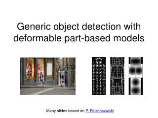
6. Famous Object Detectors (2) Felzenszwalb et. al. (PAMI 10, CVPR 10) extend the Dalal and Triggs model to include high resolution parts with flexible location.

7. Famous Object Detectors (3) Viola and Jones (IJCV 2004) construct a weak classifier by thresholding the response of a Haar filter (computed using integral images). Weak classifiers are combined into a strong classifier using AdaBoost.

8. Outline

9. Motivation Different object classes are characterized by different features. So we want to leave the choice of features up to the user. Therefore we construct an object detector based on feature maps. Any feature detectors in any combination can be used to generate feature maps. Corners Corners + Blobs Regions Edges

10. Our Object Detector We use AdaBoost to build a strong classifier. We construct a weak classifier by thresholding the distance from a measurement point to the closest occurrence of a given feature.

11. Outline

12. Extraction of Training Data Feature maps are extracted by some external feature detectors Distance transforms are computed for each feature map (For each training window) Distances from each measurement point to the closest occurrence of the corresponding feature are concatenated into a vector

13. Training { fi}, { Ij } Cascade Strong Learner Weak Learner Decision Stump Learner Viola-Jones Cascade Construction • Require positive training examples and background images • Randomly sample background images to extract negative training examples • Loop: • Train strong classifier • Append strong classifier to current cascade • Run cascade on background images to harvest false positives • If number of false positives sufficiently few, stop { fi}, { ci }, T { fi}, { ci }, { di} { fi}, { ci }, { di}

14. Training { fi}, { Ij } Cascade Strong Learner Weak Learner Decision Stump Learner Viola-Jones Cascade Construction • Require positive training examples and background images • Randomly sample background images to extract negative training examples • Loop: • Train strong classifier • Append strong classifier to current cascade • Run cascade on background images to harvest false positives • If number of false positives sufficiently few, stop { fi}, { ci }, T { fi}, { ci }, { di} { fi}, { ci }, { di}

15. Training { fi}, { Ij } Cascade Strong Learner Weak Learner Decision Stump Learner AdaBoost • Require labeled training examples and number of rounds • Init. weights of training examples • For each round • Train weak classifier • Compute weight of weak classifier • Update weights of training examples { fi}, { ci }, T { fi}, { ci }, { di} { fi}, { ci }, { di}

16. Training { fi}, { Ij } Cascade Strong Learner Weak Learner Decision Stump Learner AdaBoost • Require labeled training examples and number of rounds • Init. weights of training examples • For each round • Train weak classifier • Compute weight of weak classifier • Update weights of training examples { fi}, { ci }, T { fi}, { ci }, { di} { fi}, { ci }, { di}

17. Training { fi}, { Ij } Cascade Strong Learner Weak Learner Decision Stump Learner Decision Tree Learner Require labeled and weighted training examples Compute node output Train decision stump Split training examples using decision stump Evaluate stopping conditions Train decision tree on left subset of training examples Train decision tree on right subset of training examples { fi}, { ci }, T { fi}, { ci }, { di} { fi}, { ci }, { di}

18. Training { fi}, { Ij } Cascade Strong Learner Weak Learner Decision Stump Learner Decision Tree Learner Require labeled and weighted training examples Compute node output Train decision stump Split training examples using decision stump Evaluate stopping conditions Train decision tree on left subset of training examples Train decision tree on right subset of training examples { fi}, { ci }, T { fi}, { ci }, { di} { fi}, { ci }, { di}

19. Training { fi}, { Ij } Cascade Strong Learner Weak Learner Decision Stump Learner Feature and Threshold Selection • Require labeled and weighted training examples • For each measurement point • Compute a threshold by assuming exponentially distributed distances • Compute classification error after split • If error lower than previous errors, store threshold and measurement point { fi}, { ci }, T { fi}, { ci }, { di} { fi}, { ci }, { di}

20. Outline

21. Hierarchical Detection Evaluate an “optimistic” classifier on regions in search space. Split positive regions recursively.

22. Hierarchical Detection Evaluate an “optimistic” classifier on regions in search space. Split positive regions recursively.

23. Hierarchical Detection Evaluate an “optimistic” classifier on regions in search space. Split positive regions recursively.

24. Hierarchical Detection Evaluate an “optimistic” classifier on regions in search space. Split positive regions recursively.

25. Hierarchical Detection Evaluate an “optimistic” classifier on regions in search space. Split positive regions recursively.

26. Hierarchical Detection Evaluate an “optimistic” classifier on regions in search space. Split positive regions recursively.

27. Hierarchical Detection Each point in search space corresponds to a window in the image. In the image is a measurement point. Search space Image space s y y s x x

28. Hierarchical Detection A region in search space corresponds to a set of windows in the image. This translates to a set of locations for the measurement point. Search space Image space s y y x x

29. Hierarchical Detection We can then compute upper and lower bounds for the distance to the closest occurrence of the corresponding feature. Based on these bounds we construct an optimistic classifier. Search space Image space s y y x x

30. Outline

31. Experiments • Detection results obtained on the ETHZ Shape Classes dataset, which was used for testing only • Training data downloaded from Google images : 106 applelogos, 128 bottles, 270 giraffes, 233 mugs and 165 swans • Detections counted as correct if Aintersect/ Aunion ≥ 0.2 • Features used: edges, corners, blobs, Kadir-Brady + SIFT + quantization

32. Results Real AdaBoost slightly better than Dirscrete and Gentle AdaBoost

33. Results Decision tree weak classifiers should be shallow

34. Results Using all features are better than using only edges

35. Results Using the asymmetric weighting scheme of Viola and Jones yields a slight improvement

36. Results Applelogos Mugs Bottles Swans

37. Results Hierarchical search yields a significant speed-up

38. Outline

39. Conclusion • Proposed object detection scheme based on feature maps • Used distances from measurement points to nearest feature occurrence in image to construct weak classifiers for boosting • Showed promising detection performance on the ETHZ Shape Classes dataset • Showed that a hierarchical detection scheme can yield significant speed-ups • Thanks for listening!

40. Famous Object Detectors (4) Laptev (IVC 09) construct a weak classifier using a linear discriminant on a histogram of oriented gradients (HOG – computed by integral histograms) from a sub-region of the window. Again, weak classifiers are combined into a strong classifier using AdaBoost.