Download
1 / 31
310 likes | 477 Views
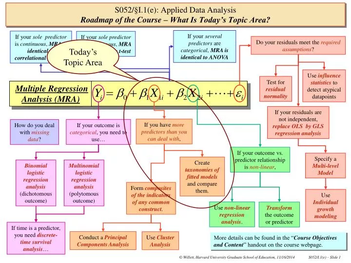
If your several predictors are categorical , MRA is identical to ANOVA. If your sole predictor is continuous , MRA is identical to correlational analysis. If your sole predictor is dichotomous , MRA is identical to a t-test. Do your residuals meet the required assumptions ?.

E N D
If your several predictors are categorical, MRA is identical to ANOVA If your sole predictor is continuous, MRA is identical to correlational analysis If your solepredictor is dichotomous, MRA is identical to a t-test Do your residuals meet the required assumptions? Today’s Topic Area Use influence statistics to detect atypical datapoints Test for residual normality Multiple Regression Analysis (MRA) If your residuals are not independent, replace OLS byGLS regression analysis If you have more predictors than you can deal with, If your outcome is categorical, you need to use… How do you deal with missing data? If your outcome vs. predictor relationship isnon-linear, Specify a Multi-level Model Create taxonomies of fitted models and compare them. Binomiallogistic regression analysis (dichotomous outcome) Multinomial logistic regression analysis (polytomous outcome) Form composites of the indicators of any common construct. Use Individual growth modeling Use non-linear regression analysis. Transform the outcome or predictor If time is a predictor, you need discrete-time survival analysis… Conduct a Principal Components Analysis Use Cluster Analysis More details can be found in the “Course Objectives and Content” handout on the course webpage. S052/§I.1(e): Applied Data AnalysisRoadmap of the Course – What Is Today’s Topic Area?
Syllabus Section I.1(e), on Interpreting Findings, includes: • Three things you must report, in a statistical analysis (Slide 3). • The difference between analysis & reporting (Slide 4). • Deciding what to report (Slides 5-6). • Sidelining an effect by setting a predictor to a prototypical value (Slide 7). • Plotting fitted trend lines for prototypical children, and crafting a conclusion (Slide 8-13). • Using the GLH strategy to test “post-hoc” hypotheses (Slides 14-18). • Carrying out the “post-hoc” GLH test by hand (Slides 19-21). • Appendix 1: Main effects of multiple dummies (Slides 22-25). • Appendix 2: Interactions with multiple dummies (Slides 26-29). • Appendix 3: What happens to main effects when interactions are added? (Slides 30-31). S052/§I.1(e): Applied Data AnalysisPrinted Syllabus – What Is Today’s Topic? Please check inter-connections among the Roadmap, the Daily Topic Area, the Printed Syllabus, and the content of today’s class when you pre-read the day’s materials.
Report whether you have detected an effect, or not. Report the magnitude of the effectyou have detected. Report the direction of the effect you have detected Stipulate whether the effect is small, medium, or large. • Report your hypothesis testingto stipulate whether the effect isdifferent from zero in the population. Stipulate whether the effect is positive or negative? • When you report differences between groups, a difference of: • .2 st. dev. is small • .5 st. dev. is medium • .8 st. dev. is large • When you report relationships, a correlation of : • .10 is small • .30 is medium • .50 is large You can often achieve all this simultaneously, by plotting fitted trend linesforindividuals who are prototypical for the population. When you report your analyses, You must address three important things S052/§I.1(e): Interpreting FindingsThree Things You Must Include, In The Report Of Any Statistical Analysis
“ANALYSIS” • In analysis, you must include all important effectsin your hypothesized regression models: • If you don’t, then you may not have represented the underlying population process credibly. • “REPORTING” • In reporting, you don’t need to report every effect included in your analysis: • Focus on the main story and present evidence selected to tell that story in the most effective way. • Need not report effects you’ve detected in the same form in which they were specified in the analyses (and vice versa!): • Can always conduct additional GLH tests to check out interesting post-hoc hypotheses. Effective reporters? Your report (thesis, paper, presentation) is NOT a “A Diary of the Data-Analysis I Did Last Summer” In your work, make sure you distinguish carefully between… S052/§I.1(e): S052/§I.1(e): Interpreting FindingsWhich Leads To An Obvious, But Critically Important Distinction!!! • Possible structure for a: • Research Proposal • Journal Article • Conference Presentation
We’ll report the “final” model, of course. But, to decide whether there are others that should be reported too, ask: • Do we want to tell more than one story? • Which stories will we forefront, which background? • Which model(s) supports the story we want to forefront? Which the one we want to background? • Should we alert the audience to particular models that were key links in the analytic chain? • Is there a model that a particular audience would “expect” to see in our report? • When the refrigerator door is closed and the little light goes out, do the vegetables get scared in the dark? • …? These were the models that I fitted in order to get to the “final” model … But, which ones should I report … ? S052/§I.1(e): Interpreting Findings You’ve Done The Analysis, But What Should You Report?
Before we get to the actual report, let’s think about how best to interpret the main and interaction effects in this “final” model in the taxonomy. Here’s one possible subset of the taxonomy that we could effectively report, in a journal article or thesis … S052/§I.1(e): Interpreting Findings Deciding What We Should Report!
The “hat” over the outcome variable indicates that this is the equation for the predicted values, and so this must be the fitted model. Notice that there is no residual term in a fitted model. The fitted model contains all the important effects detected, butwhich effects should feature in the interpretation? We must interpretthe effect of health status (H) -- it’s the question predictor. We should interprettheeffect of AGE, because theP.I. had a “developmental” interest in the children? Perhaps we don’t need to interpret theeffect of SES – because it was only included as a covariate to ensure that the “health” story was captured correctly? • How to present findings, without interpreting SES? • Don’t ignore SES, just set it to some sensibleprototypical value: • Perhaps the sample mean -- here, 2.3 (Handout I_1e_1)? • Or, to some other substantively-reasonable value? • How is this done? • Substitute this value for SES in the fitted model, & simplify. • Proceed with interpretation of remaining effects as usual. • But, describe them as applying to a “child of average SES.” S052/§I.1(e): Interpreting Findings Algebraic Representation of the “Final” Fitted Model … What Should We Interpret?
This notation indicates that the fitted values of the outcome are now expressed at the “prototypical” substituted value of SES(= 2.3) We can interpret this new specification of the fitted model to illustrate the simultaneous impact of ILL and AGE for children of average SES. Let’s try this – set SES to its sample average (2.3), and simplify & collect terms in the fitted model … S052/§I.1(e): Interpreting Findings Sidelining A Detected Effect By Setting The PredictorTo A Prototypical Value Make Sure You Can Explain The Steps Illustrated On This Page, In Words.
Fitted values of ILLCAUSE (computed at the average value of SES) will be plotted on the vertical axis (ordinate). • Create a fitted plot in which AGE is plotted along the horizontal axis, and there are two fitted regression lines: • One for chronically-ill children (ILL=1), • One for healthychildren (ILL=0). So, here’s the new version of the final fitted model for a prototypical child of average SES (=2.3) … S052/§I.1(e): Interpreting Findings Figuring Out Which Fitted Lines To Plot, For The Children Of Average SES? And here are the fitted models representing the required fitted trend lines that we must plot: Healthy, Average SES Chronically Ill, Average SES Can You Explain The Steps In The Process Illustrated On This Page, In Words?
Age (months) Min Max Ill 61 200 Healthy 64 203 Figure I.1(e).1. Predicted understanding of illness causality as a function of child age (in months) by health status, for children of average socio-economic status (SES=2.3). Healthy S052/§I.1(e): Interpreting Findings Plotting the Fitted Lines For Prototypical Children Chronically Ill Do You Know How To Use MS Excel To Create Such Plots?
It may be important to show the impact of SES on the outcome, along with the impact of HEALTH and AGE (it would be even more important if SES had interacted with other predictors in the model!) • “Hi SES” Plot • Fitted ILLCAUSE vs AGE, • For Healthy & Ill children • “Lo SES” Plot • Fitted ILLCAUSE vs AGE, • For Healthy & Ill children S052/§I.1(e): Interpreting Findings How Would You Include The Effect Of SES Explicitly In The Interpretation? • The main effect of SES can be surfaced explicitly by: • Using the earlier approach to interpreting the effects of ILL and AGE, but offering them at contrasting prototypical values of SES. • For example, at the 25st (“Hi SES”) and 75th (“Lo SES”) percentiles of socio-economic status, say (SES=2 and 3, respectively). Panel Of Plots For Four Prototypical Children What Features Must You Consider When Deciding How To Assemble Such A Panel Of Plots?
Low socio-economic status (SES=3): S052/§I.1(e): Interpreting Findings Creating A Panel Of Plots To Display Simultaneous Effects Of HEALTH, AGE & SES High socio-economic status (SES=2): Can You Explain The Steps In The Process Illustrated On This Page, In Words?
Figure I.1(e).2. Fitted values of understanding of illness causality versus the child’s age (in months) by health status, for children of low (SES=3) and high (SES=2) socio-economic status. SES=2 SES=3 S052/§I.1(e): Interpreting Findings Panel Of Plots To Display Simultaneous Effects Of HEALTH, AGE & SES SES=2 SES=3 Healthy Chronically Ill What Conclusion Would You Craft To Accompany This Panel Of Plots?
Whichever way you plot them and whatever stories you decide to tell … inspection of fitted plots often suggests interesting follow-up questions whose answers may provide a useful perspective in your written account! Healthy S052/§I.1(e): Interpreting Findings Generating Interesting Post-Hoc Questions About Detected Effects e.g., because the ILL×AGE interaction is present in the fitted model, differences between healthy and chronically ill children in the predicted values of ILLCAUSEare greater among older children. This does not mean, however, that there are statistically significant differences between healthy and ill children at every age! Chronically Ill For instance, perhaps children of average SES really start off their lives understanding illness at the same levels regardless of their their health status (on average, in the population)? Perhaps there are really no differences between healthy and ill children (of average SES) when they are young, at 60 months, say? You can provide an answer to a “post-hoc” question like this by conducting a General Linear Hypothesis Test.
This is called theStructural Partof the right hand side of the hypothesized regression model, because it contains our hypotheses about the structure of the underlying population process. We often write it out separately as: This is called the Stochastic partof the hypothesized regression model, because it contains our hypotheses about the randomness in the underlying population This “Expectation” notation – represented by E[…] – indicates that we are concerned with the average value of the outcome for different types of folk in the population, as designated by their ILL, AGE & SES values. If we are postulating and testing hypotheses about population process, we use the structural part of the model to express our hypotheses about the expected value of the outcome … Let’s conduct a GLH test to determine whether the value of ILLCAUSE at age-60 months is the samefor healthy andchronically-ill children, on average, in the population ... To do this, we must first work with the hypothesized, not the fitted, final model to figure out the algebraic form of the null hypothesisthat we must test in order to address our post-hoc question … we start, therefore, with: S052/§I.1(e): Interpreting Findings Testing More Complex Post-Hoc Hypotheses:Distinguishing Structural and Stochastic Parts of the Hypothesized Regression Model
These two expressions are the hypothesized population values of ILLCAUSE for the two types of prototypical children … let’s carry them forward … We use the “expectation” form of the hypothesized regression model to figure out a null hypothesis that we can test, to address our post-hoc question about the possible equivalence of the values of ILLCAUSE for chronically-ill andhealthy children atage60 months, on average, in the population … as follows S052/§I.1(e): Interpreting Findings Does the Understanding Of Illness Causality of Healthy ChildrenDiffer From That Of Chronically Ill Children, When They Are Young? First, let’s substitute chosen prototypical values of the predictors into the structural part of the model to specify the particular groups of children whose values of ILLCAUSE we want to compare, on average, in the population … they are: Healthy (ILL=0) children of avg.socio-economic status (SES=2.3) at age 60 months (AGE=60): Chronically-ill (ILL=1) children of avg. socio-economic status (SES=2.3) at age 60 months (AGE=60):
Healthy, 60 months, avg. SES Healthy S052/§I.1(e): Interpreting Findings Does the Understanding Of Illness Causality of Healthy ChildrenDiffer From That Of Chronically Ill Children, When They Are Young? Chronically Ill And here’s the focus of our GLH test … we must test: Chronically ill, 60 months, avg. SES So, the difference in the population values of ILLCAUSE between the chronically ill and healthy groups at age=60 and avg. SES
Test: Results for Dependent Variable ILLCAUSE Mean Source DF Square F Value Pr > F Numerator 1 1.41407 4.06 0.0452 Denominator 189 0.34803 Since p<.05, reject: Conclude that the understanding of illness causality of chronically ill and healthy children, of average SES, is not the same at age-60 months, on average in the population. While this appears complex, it can actually be handled easily by the General Linear Hypothesis testing strategy introduced earlier … the new test is carried out in Data-Analytic Handout I.1(e).2, as follows: *-----------------------------------------------------------* Use a GLH test to address an interesting post-hoc question *-----------------------------------------------------------*; * Here's the final "full" model, yet again; PROC REG DATA=ILLCAUSE; VAR ILLCAUSE ILL AGE SES; M6F: MODEL ILLCAUSE = ILL AGE ILLxAGE SES; * Here's the post-hoc test; TEST ILL + 60*ILLxAGE = 0; S052/§I.1(e): Interpreting Findings Does the Understanding Of Illness Causality of Healthy ChildrenDiffer From That Of Chronically Ill Children, When They Are Young?
Here’s our Full Model: S052/§I.1(e): Interpreting Findings Does the Understanding Of Illness Causality of Healthy ChildrenDiffer From That Of Chronically Ill Children, When They Are Young? And here’s the Null Hypothesis we want to test: • Since we know that the Reduced Model is just the Full Model with the Null Hypothesis forced into it as a Constraint … why don’t we just go ahead and “force” the null hypothesis into the full model: • You can see what this means by writing out the Full Model with the exact combination of parameters specified in the null hypothesis – that’s ILL + 60ILL×AGE -- forced to be zero within the model. • How is this done? By setting ILL equal to - 60ILL×AGEin the model, like this … As with any GLH strategy, you can always do the same test by hand – because it’s all about comparing the fit of competing models… and, even though you need not do it by hand, it is worth knowing how! The Challenge Is Figuring Out What Should Serve as the Reduced Model for this Post-Hoc Test! Reduced Model: This tells us that, if we go into the dataset, form a new composite predictor whose values are equal to the value of “ILL times AGE, minus 60 times ILL” for each child, and then we regress ILLCAUSE on: (a) AGE, (b) the new predictor, and (c) SES, we will have fitted the requisite reduced model … and can conduct the GLH test by hand!
* Create composite predictor, COMPVAR, to include in reduced model; DATA ILLCAUSE; SET ILLCAUSE; COMPVAR = ILLxAGE-(60*ILL); * Fit the reduced model; PROC REG DATA=ILLCAUSE; VAR ILLCAUSE ILL AGE SES; M6R: MODEL ILLCAUSE = AGE COMPVAR SES; Here, I create the new composite predictor, COMPVAR. S052/§I.1(e): Interpreting Findings Does the Understanding Of Illness Causality of Healthy ChildrenDiffer From That Of Chronically Ill Children, When They Are Young? And add it, along with AGE and SES, as a predictor of ILLCAUSE in order to obtain the fitted Reduced Model. Here’s the corresponding regression output: Analysis of Variance Sum of Mean Source DF Squares Square F Value Pr > F Model 3 134.35548 44.78516 126.64 <.0001 Error 190 67.19166 0.35364 Corrected Total 193 201.54714 Parameter Estimates Parameter Standard Variable DF Estimate Error t Value Pr > |t| Intercept 1 1.91296 0.18774 10.19 <.0001 AGE 1 0.02204 0.00119 18.58 <.0001 COMPVAR 1 -0.01000 0.00115 -8.70 <.0001 SES 1 -0.12882 0.04878 -2.64 0.0090 Here’s the corresponding PC-SAS code: Critical fit statistic, from the Reduced Model is SSModel = 134.3555
We can check whether the difference is “statistically significant” by converting these differences in SSModel and dfModel into an F-statistic, as usual: And because Fobserved is larger than critical value, Fcritical = F1,189(=.05) = 3.89, we can reject H0: βILL+ 60 βILLAGE= 0 S052/§I.1(e): Interpreting Findings Does the Understanding Of Illness Causality of Healthy ChildrenDiffer From That Of Chronically Ill Children, When They Are Young? Key Question: Is losing 1.414 units of fit from SSModel worth gaining 1 extra degree of freedom? The constraint that was imposed to make the full model become the reduced model is actually a statement of the null hypothesis being tested. And the GLH test can be carried out by the comparison of fits of full and reduced models, as usual … This is the observed F-statistic provided by the GLH test. This is the critical F-statistic implicit in the GLH test. The “denominator” df are those of the residual variance in the full model.
Estimated slopes associated with the health status dummies describe the differences in average predicted ILLCAUSEbetween diabetic & healthy childrenand between asthmatic & healthy children, respectively Estimated intercept tells you the average predicted ILLCAUSE for healthy children For pedagogic simplicity, let’s consider a model that is not the final model in the taxonomy, Model M2, and ask: How can you get three fitted lines from a fitted regression model that contains only the main effects of two health status dummies, D & A (and the predictor AGE)? You proceed as follows: S052/§I.1(e): Interpreting FindingsAppendix 1: Understanding the Main Effects of Multiple Dummies • It’s easy to recover three fitted lines that describe this relationship. You just substitute appropriate values for the health status dummies, as follows: • For prototypical Healthy children, substitute D = 0 and A = 0. • For prototypical Diabetic children, substitute D = 1 and A = 0. • For prototypical Asthmatic children, substitute D = 0 and A = 1.
Healthy Child (D=0;A=0): Diabetic Child (D=1;A=0): Asthmatic Child (D=0;A=1): Plot these! Substitute the prototypical values of D and A into the fitted model: S052/§I.1(e): Interpreting Findings Appendix 1: Understanding the Main Effects of Multiple Dummies
S052/§I.1(e): Interpreting Findings Appendix 1: Understanding the Main Effects of Multiple Dummies Healthy Asthmatic Diabetic
Healthy Child (D=0;A=0): Diabetic Child (D=1;A=0): Asthmatic Child (D=0;A=1): Intercepts differ by the main effects of the health status dummies AGE-slopes identical in all three population models. You can obtain a similar explanation by substituting prototypical values of D and A into the population model… S052/§I.1(e): Interpreting Findings Appendix 1: Understanding the Main Effects of Multiple Dummies
Presence of this two-way HEALTH by AGE interaction ensures that: Either the relationship between ILLCAUSE and HEALTH differs by AGE Or the relationship between ILLCAUSE and AGE differs by HEALTH • It’s easy to recover the three fitted lines that describe this interaction, by substituting appropriate values for the health status dummies, as follows: • For prototypical Healthy children, set D=0 and A=0. • For prototypical Diabetic children, set D=1 and A=0. • For prototypical Asthmatic children, set D=0 and A=1. For pedagogic simplicity, let’s consider a model that is not the final model in the taxonomy, Model M3, and ask:How do you get three fitted lines with different slopes, when there are only interactions between two health status dummies, D & A, and predictor AGE in the fitted model? You proceed as follows: S052/§I.1(e): Interpreting Findings Appendix 2: Understanding Two-Way Interactions With Multiple Dummies
Healthy Child: Diabetic Child: Asthmatic Child: Plot these! Substitute the prototypical values of D and A into the fitted model: S052/§I.1(e): Interpreting Findings Appendix 2: Understanding Two-Way Interactions With Multiple Dummies
S052/§I.1(e): Interpreting Findings Appendix 2: Understanding Two-Way Interactions With Multiple Dummies Asthmatic Diabetic Healthy
Healthy Child (D=0;A=0): Diabetic Child (D=1;A=0): Asthmatic Child (D=0;A=1): AGE-slopes differ by the effects of the interactions between AGE and the health status dummies Intercepts differ by the main effects of the health status dummies A similar explanation can be obtained by substituting prototypical values of D and A into the population model… S052/§I.1(e): Interpreting Findings Appendix 2: Understanding Two-Way Interactions With Multiple Dummies
Notice the magnitudes and directions of the main effects of health status differ when the health status by AGE interaction is added to convert Model M2 into Model M3! What does this mean, or imply? It’s pretty easy to see what’s going on, if you plot prototypical trajectories for both models. For pedagogic simplicity, let’s consider models that are not the final models in the taxonomy, Models M2 and M3, and ask:Why does the interpretation of the main effects differ when an interaction term is added to the model? S052/§I.1(e): Interpreting Findings Appendix 3: What Happens to the Main Effects When Two-Way Interactions Are Included?
Situation in the middle of the data remains pretty much the same! Differences in the main effects of health status between M2 and M3 reflect the differences in intercept that occur as a result of the fitted lines “tilting” due to the presence of the Health by Age interaction S052/§I.1(e): Interpreting Findings Appendix 3: What Happens to Main Effects When Two-Way Interactions Are Included