Download

1 / 29
290 likes | 551 Views
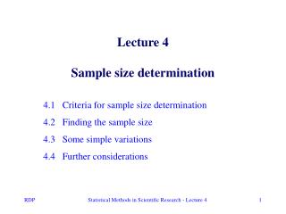
Design and Analysis of Clinical Study 4. Sample Size Determination. Dr. Tuan V. Nguyen Garvan Institute of Medical Research Sydney, Australia. Practical Difference vs Statistical Significance. Outcome Group A Group B Improved 9 18 No improved 21 12 Total 30 30

E N D
Design and Analysis of Clinical Study 4. Sample Size Determination Dr. Tuan V. Nguyen Garvan Institute of Medical Research Sydney, Australia
Practical Difference vs Statistical Significance Outcome Group A Group B Improved 9 18 No improved 21 12 Total 30 30 % improved 30% 60% Outcome Group A Group B Improved 6 12 No improved 14 8 Total 20 20 % improved 30% 60% Chi-square: 5.4; P < 0.05 “Statistically significant” Chi-square: 3.3; P > 0.05 “Statistically insignificant”
The Classical Hypothesis Testing • Define a null hypothesis (H0) and a null hypothesis (H1) • Collect data (D) • Estimate p-value = P(D | H0) • If p-value > a, accept H0; if p-value < a, reject H0
P-value là gì ? “Alendronate treatment was associated with a 5% increase in BMD compared to placebo (p<0.05)” • It has been proved that alendronate is better than placebo? • If the treatment has no effect, there is less than a 5% chance of obtaining such result • The observed effect is so large that there is less than 5% chance that the treatment is no better than placebo • I don’t know
P value is NOT • the likelihood that findings are due to chance • the probability that the null hypothesis is true given the data • P-value is 0.05, so there is 95% chance that a real difference exists • With low p-value (p < 0.001) the finding must be true • The lower p-value, the stronger the evidence for an effect
P-value • Grew out of quality control during WWII • Question: the true frequency of bad bullets is 1%, what is the chance of finding 4 or more bad bullets if we test 100 bullets? • Answer: With some maths (binomial theorem), p=2% So, p-value is the probability of getting a result as extreme (or more extreme) than the observed value given an hypothesis
Process of Reasoning The current process of hypothesis testing is a “proof by contradiction” If the null hypothesis is true, then the observations are unlikely. The observations occurred ______________________________________ Therefore, the null hypothesis is unlikely If Tuan has hypertension, then he is unlikely to have pheochromocytoma. Tuan has pheochromocytoma ______________________________________ Therefore, Tuan is unlikely to have hypertension
What do we want to know? • Clinical P(+ve | Diseased): probability of a +ve test given that the patient has the disease P(Diseased | +ve): probability of that the patient has the disease given that he has a +ve test • Research P(Significant test | No association): probability that the test is significant given that there is no association P(Association | Significant test): probability that there is an association given that the test statistic is significant
Case study • Một phụ nữ 45 tuổi • Không có tiền sử ung thư vú trong gia đình • Đi xét nghiệm truy tầm ung thư bằng mammography • Kết quả dương tính • Hỏi: Xác suất người phụ nữ này bị ung thư là bao nhiêu? - Tần suất ung thư trong quần thể Các yếu tố liên quan cần biết để có câu trả lời: - Độ nhạy của test chẩn đoán - Độ đặc hiệu của test chẩn đoán
Giải đáp 10000 Phụ nữ Kết quả +ve= +ve mammography -ve= -ve mammography Tần suất ung thư trong quần thể: 1% Ung thư 100 Không 9900 Độ nhạy của xét nghiệm: 95% Độ đặc hiệu xét nghiệm: 90% +ve 95 -ve 5 +ve 990 -ve 8910 Tổng số bệnh nhân +ve: 95 + 990 =1085 Xác suất bị K nếu có kết quà dương tính: 95/1085= 0.087
Suy luận trong nghiên cứu khoa học 10000 nghiên cứu Vit C +ve: p <0.05 -ve: p>0.05 Vit C = giả dược, 50% Hiệu quả 5000 Không 5000 Power: 80% Alpha: 5% +ve 4000 -ve 1000 +ve 250 -ve 4750 β 1-β α 1-α Sai lầm loại II Sai lầm loại I Tổng số kết quả nghiên cứu +ve: 4000+250 =4250 Xác suất Vit C có hiệu quả vói điều kiện +ve kết quả: 4000/4250= 0.94
What Are Required for Sample Size Estimation? • Parameter (or outcome) of major interest • Blood pressure • Magnitude of difference in the parameter • 10 mmHg is an important difference / effect • Variability of the parameter • Standard deviation of blood pressure • Bound of errors (type I and type II error rates) • Type I error = 5% • Type II error = 20% (or power = 80%)
The Normal Distribution 0.95 Prob. Z1 Z2 0.80 0.84 1.28 0.90 1.28 1.64 0.95 1.64 1.96 0.99 2.33 2.81 0.95 Z2 Z1 1.64 -1.96 1.96 0 0 0.05 0.025 0.025
The Normal Deviates Alpha Za/2 c 0.20 1.28 0.10 1.64 0.05 1.96 0.01 2.81 Power Z1-b 0.80 0.84 0.90 1.28 0.95 1.64 0.99 2.33
Study Design and Outcome • Single population • Two populations • Continuous measurement • Categorical outcome • Correlation
Sample Size for Estimating a Population Proportion • How close to the true proportion • Confidence around the sample proportion. • Type I error. • N = (Za/2)2p(1-p) / d2 • p: proportion to be estimated. • d: the accuracy of estimate (how close to the true proportion). • Za/2: A Normal deviate reflects the type I error. • Example: The prevalence of obesity is thought to be around 20%. We want to estimate the preference p in a community within 1% with type I error of 5%. • Solution N = (1.96)2 (0.2)(0.8) / 0.012 = 6146 individuals.
Effect of Accuracy • Example: The prevalence of disease in the general population is around 30%. We want to estimate the prevalence p in a community within 2% with 95% confidence interval. • N = (1.96)2 (0.3)(0.7) / 0.022 = 2017 subjects.
Sample Size for Difference between Two Means • Hypotheses: Ho: m1 = m2 vs. Ha: m1 = m2 + d • Let n1and n2be the sample sizes for group 1 and 2, respectively; N = n1+ n2; r = n1/ n2;s: standard deviation of the variable of interest. • Then, the total sample size is given by: • If we let Z = d/s be the “effect size”, then: • If n1 = n2 ,power = 0.80, alpha = 0.05, then (Za + Z1-b)2 = (1.96 + 1.28)2 = 10.5, then the equation is reduced to: Where Za and Z1-b are Normal deviates
Sample Size for Two Means vs.“Effect Size” For a power of 80%, significance level of 5%
Sample Size for Difference between 2 Proportions • Hypotheses: Ho: p1 = p2 vs. Ha: p1 = p2 + d . • Let p1and p2 be the sample proportions (e.g. estimates of p1 and p2) for group 1 and group 2. Then, the sample size to test the hypothesis is: Where: n = sample size for each group ; p = (p1 + p2) / 2 ; Za and Z1-b are Normal deviates A better (more conservative) suggestion for sample size is:
Sample Size for Difference Between 2 Prevalence • For most diseases, the prevalence in the general population is small (e.g. 1 per 1000 subjects). Therefore, a difference formulation is required. • Let p1and p2 be the prevalence for population 1 and population 2. Then, the sample size to test the hypothesis is: Where: n = sample size for each group; Za and Z1-b are Normal deviates.
Sample Size for Two Proportions: Example • Example: The preference for product A is expected to be 70%, and for product B 60%. A study is planned to show the difference at the significance level of 1% and power of 90%. • The sample size can be calculated as follows: • p1= 0.6; p2= 0.7; p = (0.6 + 0.7)/2 = 0.65; Z0.01 = 2.81; Z1-0.9 = 1.28. • The sample size required for each group should be: • Adjusted / conservative sample size is:
Sample Size for Two Proportions vs. Effect Size Difference from p1 by: 0.1 0.2 0.3 0.4 0.5 0.6 0.7 0.8 P1 0.1 424 131 67 41 28 19 14 10 0.2 625 173 82 47 30 20 14 9 0.3 759 198 89 50 30 19 13 8 0.4 825 206 89 47 28 17 . . 0.5 825 198 82 41 22 . . . 0.6 759 173 67 31 . . . . 0.7 625 131 45 . . . . . 0.8 424 73 . . . . . . Note: these values are “unadjusted” sample sizes
Sample size for Estimating an Odds Ratio • In case-control study the data are usually summarized by an odds ratio (OR), rather then difference between two proportions. • If p1 and p2 are the proportions of cases and controls, respectively, exposed to a risk factor, then: • If we know the proportion of exposure in the general population (p), the total sample size N for estimating an OR is: • Where r = n1 / n2 is the ratio of sample sizes for group 1 and group2; p is the prevalence of exposure in the controls; and OR is the hypothetical odds ratio. If n1 = n2 (so that r = 1) then the fomula is reduced to:
Sample Size for an Odds Ratio: Example • Example: The prevalence of vertebral fracture in a population is 25%. It is interested to estimate the effect of smoking on the fracture, with an odds ratio of 2, at the significance level of 5% (one-sided test) and power of 80%. • The total sample size for the study can be estimated by:
Some Comments • The formulae presented are theoretical. • They are all based on the assumption of Normal distribution. • The estimator [of sample size] has its own variability. • The calculated sample size is only an approximation. • Non-response must be allowed for in the calculation.
Computer Programs • Software program for sample size and power evaluation • PS (Power and Sample size), from Vanderbilt Medical Center. This can be obtained from me by sending email to (t.nguyen@garvan.org.au). Free. • On-line calculator: • http://ebook.stat.ucla.edu/calculators/powercalc/ • References: • Florey CD. Sample size for beginners. BMJ 1993 May 1;306(6886):1181-4 • Day SJ, Graham DF. Sample size and power for comparing two or more treatment groups in clinical trials. BMJ 1989 Sep 9;299(6700):663-5. • Miller DK, Homan SM. Graphical aid for determining power of clinical trials involving two groups. BMJ 1988 Sep 10;297(6649):672-6 • Campbell MJ, Julious SA, Altman DG. Estimating sample sizes for binary, ordered categorical, and continuous outcomes in two group comparisons. BMJ 1995 Oct 28;311(7013):1145-8. • Sahai H, Khurshid A. Formulae and tables for the determination of sample sizes and power in clinical trials for testing differences in proportions for the two-sample design: a review. Stat Med 1996 Jan 15;15(1):1-21. • Kieser M, Hauschke D. Approximate sample sizes for testing hypotheses about the ratio and difference of two means. J Biopharm Stat 1999 Nov;9(4):641-50.