Download
1 / 83
830 likes | 931 Views
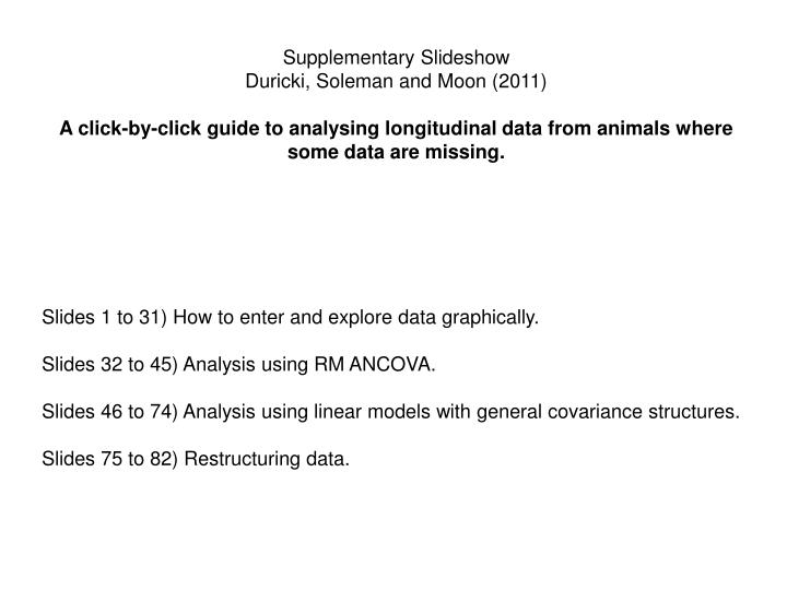
Supplementary Slideshow Duricki, Soleman and Moon (2011) A click-by-click guide to analysing longitudinal data from animals where some data are missing. Slides 1 to 31) How to enter and explore data graphically. Slides 32 to 45) Analysis using RM ANCOVA.

E N D
Supplementary Slideshow Duricki, Soleman and Moon (2011) A click-by-click guide to analysing longitudinal data from animals where some data are missing. Slides 1 to 31) How to enter and explore data graphically. Slides 32 to 45) Analysis using RM ANCOVA. Slides 46 to 74) Analysis using linear models with general covariance structures. Slides 75 to 82) Restructuring data.
Supplementary Slideshow, Slide 1: Loading data. Click “Cancel”.
Supplementary Slideshow, Slide 2: Loading data. Click File>Open>Data.
Supplementary Slideshow, Slide 3: Navigate to “short format” data file. You need to have downloaded this from Nature Protocols or www.lawrencemoon.co.uk/resources/mixedmodels.asp
Supplementary Slideshow, Slide 4: Data View Click on the “A1” icon (green circle) to toggle between label names and label numbers.
Supplementary Slideshow, Slide 5 In Variable View, click on Blue icon (“…” in green circle) to discover the names of the Levels for the Factor “group”. Missing values have been coded “999.00”
Supplementary Slideshow, Slide 6: Variable View showing four Levels for “group” Factor
Supplementary Slideshow, Slide 8 and Figure 3: Data View of “long format” data suitable for analysis using the Mixed Model>Linear procedure
Supplementary Slideshow, Slide 9: Variable View for “long format” data
Supplementary Slideshow, Slide 10: To plot individual rat performances over time, from “long format” data, click Graphs>Chart Builder
Supplementary Slideshow, Slide 11: The Warning dialog reminds you to make sure you set up the variable types in Variable View properly (i.e., select Nominal / Ordinal / Scale correctly for each variable)
Supplementary Slideshow, Slide 12: Click on “Line” then drag the icon with three lines into the “Chart preview” window
Supplementary Slideshow, Slide 14 and Figure 4: Graphs showing individual rat performances over time arranged by group and colour coded according to Subject number (rat).
Supplementary Slideshow, Slide 15: How to generate a graph of mean group performance over time.
Supplementary Slideshow, Slide 16 and Figure 5: Graphs showing mean performances over time arranged by group. Note that the last data points for AAV-NT3 and AAV-GFP do not include data from rats with missing values
Supplementary Slideshow, Slide 17: Same data but plotted with missing values replaced by Last Value Carried Forward. Data points now include all available data from all animals.
Supplementary Slideshow, Slide 18: How to determine if group variances are similar i.e., test if group variances are “heterogeneous”
Supplementary Slideshow, Slide 31: These correlations were generated without splitting the output by “group”. There is a significant and positive correlation between most pairs of time points. The size of the correlation stays similar with increasing separation of time points. This suggests that a compound symmetric (CS) covariance structure may be appropriate.
Supplementary Slideshow, Slide 34: Note that the Repeated Measure only includes the eight post-treatment time points and does not include the pre-operative baseline measurement time point (as this reduces the power of the test).
Supplementary Slideshow, Slide 37. Here’s the Syntax you generated. To obtain pairwise comparisons for the interaction, delete the full stop at the end and add these lines: /EMMEANS=TABLES(group*wave) WITH(mean_preop=MEAN)COMPARE (group) ADJ(LSD) /EMMEANS=TABLES(group*wave) WITH(mean_preop=MEAN)COMPARE (wave) ADJ(LSD).
Supplementary Slideshow, Slide 38 Ensure there is ONLY one full stop (period), at the end. Now click Run>All
Supplementary Slideshow, Slide 45: Scroll down to group * wave and then inspect pairwise comparisons