Download
1 / 60
600 likes | 636 Views
Learn the basics of linear programming to optimize resource allocation among competing activities. Follow a prototype example involving Wyndor Glass Co. in maximizing profit by producing two new products efficiently. Explore the linear programming model formulation, constraints, and graphical solution method.

E N D
Chapter 3 Introduction to Linear Programming
Introduction • Linear programming • Programming means planning • Model contains linear mathematical functions • An application of linear programming • Allocating limited resources among competing activities in the best possible way • Applies to wide variety of situations
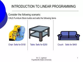
3.1 Prototype Example • Wyndor Glass Co. • Produces windows and glass doors • Plant 1 makes aluminum frames and hardware • Plant 2 makes wood frames • Plant 3 produces glass and assembles products
Prototype Example • Company introducing two new products • Product 1: 8 ft. glass door with aluminum frame • Product 2: 4 x 6 ft. double-hung, wood-framed window • Define the problem: What mix of products would be most profitable (determine the production rate of each product to maximize the profit)? • Assuming company could sell as much of either product as could be produced
Prototype Example • Products produced in batches of 20 • Data needed (data gathering process) • Number of hours of production time available per week in each plant for new products • Production time used in each plant for each batch of each new product • Profit per batch of each new product
Prototype Example • Formulating the model (decision variables, objective function and constraints) x1 = number of batches of product 1 produced per week x2 = number of batches of product 2 produced per week Z = total profit per week (thousands of dollars) from producing these two products • From bottom row of Table 3.1
Prototype Example • Constraints (see Table 3.1) • Classic example of resource-allocation problem • Most common type of linear programming problem
Prototype Example • Problem can be solved graphically • Two dimensional graph with x1 and x2 as the axes • First step: sketch the feasible region (values of x1 and x2in this region satisfy the constraint restrictions) • See Figures 3.1 and Figure 3.2 • Next step: find outa point in the feasible region that maximizes value of Z = 3x1 + 5x2 • See Figure 3.3
Prototype Example Rewrite z = 3x1 + 5x2 as x2 = -3x1/5 + z/5, the graph of this is a line with slope -3/5 and y-interception z/5. To maximize z is equivalent to maximizing the y-intercept z/5 (among all parallel line segments in the feasible region having slope -3/5). Figure 3.3 illustrates three parallel lines of different y-intercepts. Note that since |-3/5| < |-3/2| (-3/2 is the slope of the third constraint boundary), the lines of the objective function is less steep. The objective function line on the feasible region that maximizes the y-intercept is the line having the corner point (2, 6) on the line (the only point from the feasible region is on the line).
3.2 The Linear Programming Model • General problem terminology and examples • Resources: money, particular types of machines, vehicles, or personnel • Activities: investing in particular projects, advertising in particular media, or shipping from a particular source • Problem involves choosing levels of activities to maximize overall measure of performance
The Linear Programming Model • Standard form The first m constraints are called the functional constraints. The last n constraints are nonnegativity constraints.
The Linear Programming Model • Other legitimate forms • Minimizing (rather than maximizing) the objective function • Functional constraints with greater-than-or-equal-to inequality • Some functional constraints in equation form • Some decision variables may be negative
The Linear Programming Model • Feasible solution • Solution for which all constraints are satisfied • Might not exist for a given problem • Infeasible solution • Solution for which at least one constraint is violated • Optimal solution • Has most favorable value of objective function (the largest value if the objective function is to be maximized, or the smallest value if the objective function is to be minimized) • Might not exist for a given problem (no feasible solutions or unbounded Z) • Might have multiple optimal solutions
The Linear Programming Model • Corner-point feasible (CPF) solution • Solution that lies at the corner of the feasible region (note that there are corner point solutions that do not lie in the feasible region, so they are corner-point infeasible solutions).
The Linear Programming Model • Linear programming problem with feasible solution and bounded feasible region • Must have CPF solutions and optimal solution(s) • Best CPF solution must be an optimal solution
The Linear Programming Model Example: a problem having no feasible solutions
The Linear Programming Model Example: a problem having multiple optimal solutions
The Linear Programming Model Example: a problem having feasible solutions but no optimal solution (unbounded Z)
The Linear Programming Model More examples (sketch the constraint boundaries and see): • No feasible solutions: x1 ≤ 1, x2 ≤ 2, x1 + x2 ≥ 5, x1 ≥ 0, x2 ≥ 0. 2. No optimal solutions (unbounded Z): maximize Z = 3x1 + 5x2 s.t. x1 + x2 ≥ 4, x1 ≥ 0, x2 ≥ 0 3. Multiple optimal solutions: maximize Z = 2x1 + 2x2 s.t. x1 + x2 ≤ 2, x1 ≥ 0, x2 ≥ 0 All points on the line segment between (2,0) and (0, 2) on the feasible region are optimal solutions and Z = 4.
3.3 Assumptions of Linear Programming • A Linear Programming model must simultaneously satisfy all four assumptions below 1. Proportionality assumption • The contribution of each activity to the value of the objective function (or left-hand side of a functional constraint) is proportional to the level of the activity (cjxj terms or aijxj terms) • If assumption does not hold, one must use nonlinear programming (Chapter 13)
Assumptions of Linear Programming 2. Additivity • Every function in a linear programming model is the sum of the individual contributions of the activities (∑cjxj or ∑aijxj) 3. Divisibility • Decision variables in a linear programming model may have any real number values • Including noninteger values • Assumes activities can be run at fractional values
Assumptions of Linear Programming 4. Certainty • Value assigned to each parameter (cj and aij and bi) of a linear programming model is assumed to be a known constant • Seldom satisfied precisely in real applications • Sensitivity analysis used
3.4 Additional Examples • The optimal solutions of the examples in this section can be obtained by using Excel Solver (introduced in Section 3.5) and are available on the course website. • Example 1: Design of radiation therapy for Mary’s cancer treatment • Goal: select best combination of beams and their intensities to generate best possible dose distribution • Dose is measured in kilorads This is an example of a cost-benefit-trade-off problem (it seeks the best trade-off between some cost and benefits).
Example 1: Radiation Therapy Design • Linear programming model • Using data from Table 3.7
Example 1: Radiation Therapy Design • A type of cost-benefit tradeoff problem
Example 2: Regional Planning It’slike the prototype example, it’s another resource-allocation problem).
Example 3: Personnel Scheduling It’s a cost-benefit-trade-off problem.
Example 3: Personnel Scheduling Without the integer constraints, due to the special structure of the model, the optimal solution turns out to have integer values anyway.
Example 4: Distributing Goods through a Distribution Network It’s a minimum cost flow problem.
Example 4: Distributing Goods through a Distribution Network
Example 4: Distributing Goods through a Distribution Network
Example 5: Reclaiming Solid Wastes • SAVE-IT company collects and treats four types of solid waste materials • Materials amalgamated into salable products • Three different grades of product possible • Fixed treatment cost covered by grants • Objective: maximize the net weekly profit • Determine amount of each product grade • Determine mix of materials to be used for each grade
Example 5: Reclaiming Solid Wastes It’s an example of a blending problem (find the best blend of ingredients into final products to meet certain specifications).
Example 5: Reclaiming Solid Wastes • Decision variables (for i = A, B, C; j = 1,2,3,4) = number of pounds of material j allocated to product grade i per week
3.5 Formulating and Solving Linear Programming Models on a Spreadsheet • Excel and its Solver add-in • Popular tools for solving small linear programming problems