Download
1 / 71
730 likes | 1.02k Views
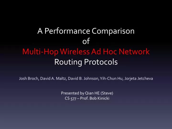
A Performance Comparison of Multi -Hop Wireless Ad Hoc Network Routing Protocols. Josh Broch , David A. Maltz , David B. Johnson, Yih -Chun Hu, Jorjeta Jetcheva. Presented by Qian HE (Steve) CS 577 – Prof. Bob Kinicki. Outline . Introduction Simulation Environment

E N D
A Performance ComparisonofMulti-Hop Wireless Ad Hoc Network Routing Protocols Josh Broch, David A. Maltz, David B. Johnson, Yih-Chun Hu, JorjetaJetcheva Presented by Qian HE (Steve) CS 577 – Prof. Bob Kinicki
Outline • Introduction • Simulation Environment • Ad Hoc Network Routing Protocols • DSDV • TORA • DSR • AODV • Methodology • Simulation Results & Observations • Conclusions
Outline • Introduction • Simulation Environment • Ad Hoc Network Routing Protocols • DSDV • TORA • DSR • AODV • Methodology • Simulation Results & Observations • Conclusions
Introduction • What is ad hoc? • Ad hoc is a Latin phrase meaning "for this". It generally signifies a solution designed for a specific problem or task, non-generalizable, and not intended to be able to be adapted to other purpose.
Introduction • What is ad hoc network? • each mobile node operates not only as a host but also as a router • ad hoc routing protocol allows each node to discover “multi-hop” paths through the network to any other node • infrastructurelessnetworking • dynamicallyestablish routing
Outline • Introduction • Simulation Environment • Ad Hoc Network Routing Protocols • DSDV • TORA • DSR • AODV • Methodology • Simulation Results & Observations • Conclusions
Simulation Environment • ns • Node mobility • A realistic physical layer including: • a radio propagation model • supporting propagation delay • capture effects • carrier sense • Radio network interfaces with properties such as: • transmission power • antenna gain • receiver sensitivity • IEEE 802.11 MAC protocol using DCF
Some details on simulation • Attenuates the power of a signal: • 1/r2at shortdistance • 1/r4at long distance • Reference distance • 100meters for outdoor • low-gain antennas 1.5 m above the groundplane • operating in the 1–2 GHz band • ARP • 50 packets with drop-tail
Outline • Introduction • Simulation Environment • Ad Hoc Network Routing Protocols • DSDV • TORA • DSR • AODV • Methodology • Simulation Results & Observations • Conclusions
Ad Hoc Network Routing Protocols • Improvements to all of the protocols: • To prevent synchronization, periodic broadcasts and packets sent in ACK were jittered using a random delay uniformly distributed between 0 and 10 milliseconds. • To insure that routing information propagated in a timely fashion, routing packets were queued for transmission at the head of the network interface. • Each of the protocols use link breakage detection feedback from the 802.11 MAC (except for DSDV).
Outline • Introduction • Simulation Environment • Ad Hoc Network Routing Protocols • DSDV • TORA • DSR • AODV • Methodology • Simulation Results & Observations • Conclusions
Destination-Sequenced Distance Vector(DSDV) • DSDV is a hop-by-hop distance vector routing protocol requiring: • each node periodically broadcast routing updates • it guarantees loop-freedom (traditional DV doesn’t) • Based on the Bellman-Ford algorithm
DSDV • Each node maintains a routing table listing the “next hop” for each reachable destination. • DSDV tags each route with a sequence number. (the higher, the better) • Each node in the network advertises a monotonically increasing even sequence number for itself. • Each node periodically broadcasts update.
DSDV Implementation • Does notuse link layer breakage detection. • Uses both full and incremental updates. • Trigger an update when: • receipt of anew sequence number for a destination will cause a triggered update (DSDV-SQ) • receipt of a new metric (simply DSDV).
Outline • Introduction • Simulation Environment • Ad Hoc Network Routing Protocols • DSDV • TORA • DSR • AODV • Methodology • Simulation Results & Observations • Conclusions
Temporally-Ordered Routing Algorithm(TORA) • A distributed routing protocol based on a “link reversal” algorithm. • Discovers routes on demand. • Provides multiple routes to a destination. • Minimizes communication overhead by localizing algorithmic reaction to topological changes. • Route optimality is considered of secondary importance. • Longer routes are often used to avoid the overhead of discovering newer routes (what?!).
TORA • Start: when a node needs a route to a particular destination, it broadcasts a QUERY packet. • Propagate: QUERY packet stops at the destination or an intermediate node having a route to the destination. • Response: the recipient then broadcasts an UPDATE packet listing its height with respect to the destination. • End: each node that receives the UPDATE sets its height to a value greater than it received.
TORA Example Node C requires a route, so it broadcasts a QRY University of Luxembourg, SECAN-Lab
TORA Example The QRY propagates until it hits a node which has a route to the destination University of Luxembourg, SECAN-Lab
TORA Example The UPD is also propagated, while node E sends a new UPD University of Luxembourg, SECAN-Lab
TORA Example Finally, every node gets its height University of Luxembourg, SECAN-Lab
TORA • TORA can be described in terms of water flowing downhill towards a destination node through a network of tubes that models the routing state of the real network.
TORA Implementation • TORA is layered on top of IMEP (Internet MANET Encapsulation Protocol). • IMEP attempts to aggregate many TORA and IMEP control together into a single packet. • Each IMEP node periodically transmits a BEACON, which is answered by each node hearing it with a HELLO. • Uses ARP instead of IMEP in network layer address resolution.
TORA Implementation • Balance overhead and routing protocol convergence: • aggregateHELLO and ACK packets for a time uniformly chosen between 150 msand 250 ms. • Does not delay TORA routing messages for aggregation. • * transmission delay of TORA routing messages + any queuing delay at the network interface, allows these routing loops to last long enough that significant numbers of data packets are dropped.
Outline • Introduction • Simulation Environment • Ad Hoc Network Routing Protocols • DSDV • TORA • DSR • AODV • Methodology • Simulation Results & Observations • Conclusions
Dynamic Source Routing(DSR) • DSR uses source routing rather than hop-by-hop routing. Each packet carries an ordered list of nodes, which the packet must pass. • intermediate nodes do not need to maintain up-to-date routing information in order to route the packets. • periodic route advertisement and neighbor detection packets are not needed. • DSR protocol consists of two mechanisms: • Route Discovery • Route Maintenance.
DSR - Route Discovery • Start: the source node broadcasts a REQUEST packet that is flooded through the network. (same as TORA, except the content of REQUEST). • Propagate: the destination node or another node that knows a route to the destination will answer with a REPLY. (same as TORA, except the content of REPLY).
DSR – Route Discovery Request: (source, request, {hops}) University of Luxembourg, SECAN-Lab
DSR – Route Discovery Reply: (source, request, route) University of Luxembourg, SECAN-Lab
DSR - Maintenance • Detectswhen the topology of the network has changed: • source node is notified with a ROUTE ERROR packet. • Decides: • if an alternative route can be used. • if the Route Discovery protocol must be started to find a new path.
DSR Implementation • Discoversonly routes composed of bidirectional links • by requiring nodes to return ROUTE REPLY messages to where ROUTE REQUEST packet came. • A node sends a ROUTE REQUEST with TTL=0. If this non-propagating search times out, it will send a propagating ROUTE REQUEST.
Outline • Introduction • Simulation Environment • Ad Hoc Network Routing Protocols • DSDV • TORA • DSR • AODV • Methodology • Simulation Results & Observations • Conclusions
Ad Hoc On-Demand Distance Vector(AODV) • AODV is essentially a combination of both DSR and DSDV. • It borrows the basic on-demand mechanism of Route Discovery and Route Maintenance from DSR. • It uses hop-by-hop routing, sequence numbers, and periodic beacons from DSDV.
AODV • Start & propagate: same as DSR, except the REQUEST contains the last known sequence number for that destination. • Response: when the REQUEST reaches a node with a route to D, it generates a REPLY that contains: • the number of hops necessary to reach D • the sequence number for D most recently seen it. • End: Each node that participates in forwarding this REPLY back toward S, creates a forward route to D by remembering only the next hop (same as DSDV).
AODV - Maintenance • Each node periodically transmit a HELLOmessage with a default rate of once per second. • Failure to receive three consecutive HELLO messages from a neighbor ?= the neighbor is down. • Alternatively, may use physical layer or link layer methods to detect link breakages. • UNSOLICITED REPLY containing an infinite metric for that destination will be sent to any upstream node that has recently forwarded packets to a destination using that link.
AODV Implementation • also implemented a version of AODV that we call AODV-LL (link layer), using only link layer feedback from 802.11 as in DSR. • Changed AODV implementation to use a shorter timeout of 6 seconds before retrying a REQUESTfor which no REPLYhas been received (RREP WAIT TIME).
Outline • Introduction • Simulation Environment • Ad Hoc Network Routing Protocols • DSDV • TORA • DSR • AODV • Methodology • Simulation Results & Observations • Conclusions
Methodology • The overall goal of our experiments was to measure the ability of the routing protocols to react to network topology changes while continuing to successfully deliver data packets to their destinations.
Methodology • 50wireless nodes, moving about over a rectangular (1500m * 300m) flat space, simulated 900 s • 210 different scenario files with varying movement patterns and traffic loads • Physical radio characteristics: Lucent WaveLANdirect sequence spread spectrum radio.
Methodology • Movement Model • Communication Model • Scenario Characteristics • Metrics
Movement Model • “random waypoint” model • begins by remaining stationary for a pause time • selectsa random destination • movesto that destination at a speed distributed uniformly 0~MAX • upon reaching, pauses again for a pause time • repeats from 2
Movement Model • 7 different pause times: 0, 30, 60, 120, 300, 600, and 900 s. • 70different movement patterns, 10 for each value of pause time • 2 different maximum speeds: • 20 m/s • 1 m/s
Methodology • Movement Model • Communication Model • Scenario Characteristics • Metrics
Communication Model • Constant Bit Rate (CBR) • sending rates of 1, 4, and 8 packets per second • networks containing 10, 20, and 30 CBR sources • packet sizes of 64 and 1024 bytes • did not use TCP (because it’s so GOOD!!)
Methodology • Movement Model • Communication Model • Scenario Characteristics • Metrics
Scenario Characteristics • An internal mechanism of the simulator calculates the shortest path between the originated packet’s sender and its destination. • The shortest path is calculated based on a range of 250m for each radio without congestion and interference. • The average hops is 2.6, and the farthest is 8.