Download
1 / 36
370 likes | 615 Views
Introductory Control Theory. CS 659 Kris Hauser. Control Theory. The use of feedback to regulate a signal. Desired signal x d. Controller. Control input u. Signal x. Plant. Error e = x-x d (By convention, x d = 0). x’ = f(x,u). What might we be interested in?.

E N D
Introductory Control Theory CS 659 Kris Hauser
Control Theory • The use of feedback to regulate a signal Desired signal xd Controller Control input u Signal x Plant Error e = x-xd (By convention, xd = 0) x’ = f(x,u)
What might we be interested in? • Controls engineering • Produce a policy u(x,t), given a description of the plant, that achieves good performance • Verifying theoretical properties • Convergence, stability, optimality of a given policy u(x,t)
Agenda • PID control • LTI multivariate systems & LQR control • Nonlinear control & Lyapunovfuncitons • Control is a huge topic, and we won’t dive into much detail
Model-free vsmodel-based • Two general philosophies: • Model-free: do not require a dynamics model to be provided • Model-based: do use a dynamics model during computation • Model-free methods: • Simpler • Tend to require much more manual tuning to perform well • Model-based methods: • Can achieve good performance (optimal w.r.t. some cost function) • Are more complicated to implement • Require reasonably good models (system-specific knowledge) • Calibration: build a model using measurements before behaving • Adaptive control: “learn” parameters of the model online from sensors
PID control • Proportional-Integral-Derivative controller • A workhorse of 1D control systems • Model-free
Proportional term Gain • u(t) = -Kp x(t) • Negative sign assumes control acts in the same direction as x x t
Integral term Integral gain • u(t) = -Kp x(t) - KiI(t) • I(t) = (accumulation of errors) x t Residual steady-state errors driven asymptotically to 0
Instability • For a 2nd order system (momentum), P control Divergence x t
Derivative term Derivative gain • u(t) = -Kp x(t) – Kd x’(t) x
Putting it all together • u(t) = -Kp x(t) - KiI(t) - Kd x’(t) • I(t) =
Example: Damped Harmonic Oscillator • Second order time invariant linear system, PID controller • x’’(t) = A x(t) + B x’(t) + C + D u(x,x’,t) • For what starting conditions, gains is this stable and convergent?
Stability and Convergence • System is stable if errors stay bounded • System is convergent if errors -> 0
Example: Damped Harmonic Oscillator • x’’ = A x + B x’ + C + D u(x,x’) • PID controller u = -Kp x –Kd x’ – Ki I • x’’ = (A-DKp) x + (B-DKd) x’ + C - D Ki I
Homogenous solution • Instable if A-DKp > 0 • Natural frequency w0 = sqrt(DKp-A) • Damping ratio z=(DKd-B)/2w0 • If z > 1, overdamped • If z < 1, underdamped (oscillates)
Example: Trajectory following • Say a trajectory xdes(t) has been designed • E.g., a rocket’s ascent, a steering path for a car, a plane’s landing • Apply PID control • u(t) = Kp (xdes(t)-x(t)) - KiI(t) + Kd(x’des(t)-x’(t)) • I(t) = • The designer of xdes needs to be knowledgeable about the controller’s behavior! x(t) xdes(t) x(t)
Controller Tuning Workflow • Hypothesize a control policy • Analysis: • Assume a model • Assume disturbances to be handled • Test performance either through mathematical analysis, or through simulation • Go back and redesign control policy • Mathematical techniques give you more insight to improve redesign, but require more work
Multivariate Systems • x’ = f(x,u) • x X Rn • u U Rm • Because m n, and variables are coupled, this is not as easy as setting n PID controllers
Linear Time-Invariant Systems • Linear: x’ = f(x,u,t) = A(t)x + B(t)u • LTI: x’ = f(x,u) = Ax + Bu • Nonlinear systems can sometimes be approximated by linearization
Convergence of LTI systems • x’ = A x + B u • Let u = - K x • Then x’ = (A-BK) x • The eigenvaluesli of (A-BK) determine convergence • Each li may be complex • Must have real component between (-∞,0]
Linear Quadratic Regulator • x’ = Ax + Bu • Objective: minimize quadratic cost xTQ x + uTR u dtOver an infinite horizon Error term “Effort” penalization
Closed form LQR solution • Closed form solutionu = -K x, with K = R-1BP • Where P is a symmetric matrix that solves the Riccati equation • ATP + PA – PBR-1BTP + Q = 0 • Derivation: calculus of variations • Packages available for finding solution
Nonlinear Control • General case: x’ = f(x,u) • Two questions: • Analysis: How to prove convergence and stability for a given u(x)? • Synthesis: How to find u(t) to optimize some cost function?
Toy Nonlinear Systems Cart-pole Acrobot Mountain car
Proving convergence & stability with Lyapunov functions • Let u = u(x) • Then x’ = f(x,u) = g(x) • Conjecture a Lyapunov function V(x) • V(x) = 0 at origin x=0 • V(x) > 0 for all x in a neighborhood of origin V(x)
Proving stability with Lyapunov functions • Idea: prove that d/dt V(x) 0 under the dynamics x’ = g(x) around origin V(x) t g(x) t d/dt V(x)
Proving convergence with Lyapunov functions • Idea: prove that d/dt V(x) < 0 under the dynamics x’ = g(x) around origin V(x) t g(x) t d/dt V(x)
Proving convergence with Lyapunov functions • d/dt V(x) = dV/dx(x) dx/dt(x) = V(x)T g(x) < 0 V(x) t g(x) t d/dt V(x)
How does one construct a suitable Lyapunov function? • Typically some form of energy (e.g., KE + PE) • Some art involved
Direct policy synthesis: Optimal control • Input: cost function J(x), estimated dynamics f(x,u), finite state/control spaces X, U • Two basic classes: • Trajectory optimization: Hypothesize control sequence u(t), simulate to get x(t), perform optimization to improve u(t), repeat. • Output: optimal trajectory u(t) (in practice, only a locally optimal solution is found) • Dynamic programming: Discretize state and control spaces, form a discrete search problem, and solve it. • Output: Optimal policy u(x) across all of X
Discrete Search example • Split X, U into cells x1,…,xn, u1,…,um • Build transition function xj= f(xi,uk)dt for all i,k • State machine with costs dt J(xi) for staying in state I • Find u(xi) that minimizes sumof total costs. • Value iteration: repeateddynamic programming overV(xi) = sum of total futurecosts Value function for 1-joint acrobot
Receding Horizon Control (aka model predictive control) ... horizon h horizon 1
Controller Hooks in RobotSim • Given a loaded WorldModel • sim= Simulator(world) • c = sim.getController(0) • By default, a trajectory queue, PID controller • c.setMilestone(qdes) – moves smoothly to qdes • c.addMilestone(q1), c.addMilestone(q2), … – appends a list of milestones and smoothly interpolates between them. • Can override behavior to get a manual control loop. At every time step, do: • Readq,dq with c.getSensedConfig(), c.getSensedVelocity() • For torque commands: • Compute u(q,dq,t) • Send torque command via c.setTorque(u) • OR for PID commands: • Compute qdes(q,dq,t), dqdes(q,dq,t) • Send PID command via c.setPIDCommand(qdes,dqdes)
Next class • Motion planning • Principles Ch 2, 5.1, 6.1