Ordinary Differential Equations (ODEs)

1. Ordinary Differential Equations (ODEs) Daniel BaurETH Zurich, Institut für Chemie- und BioingenieurwissenschaftenETH Hönggerberg / HCI F128 – ZürichE-Mail: daniel.baur@chem.ethz.chhttp://www.morbidelli-group.ethz.ch/education/index Daniel Baur / Numerical Methods for Chemical Engineers / Explicit ODE Solvers

2. Problem Definition • We are going to look at initial value problems of explicit ODE systems, which means that they can be cast in the following form Daniel Baur / Numerical Methods for Chemical Engineers / Explicit ODE Solvers

3. Higher Order ODEs • Higher order explicit ODEs can be cast into the first order form by using the following «trick» • Therefore, a system of ODEs of order n can be reduced to first order by adding n-1 variables and equations • Example: Daniel Baur / Numerical Methods for Chemical Engineers / Explicit ODE Solvers

4. ODEs as vector field • Since we know the derivatives as function of time and solution, we can calculate them at every point in time and space Daniel Baur / Numerical Methods for Chemical Engineers / Explicit ODE Solvers

5. ODE systems as vector fields • We can do the same for ODEs systems with two variables, at a certain time point Daniel Baur / Numerical Methods for Chemical Engineers / Explicit ODE Solvers

6. Example: A 1-D First Order ODE • Consider the following initial value problem • This ODE and its solution follow a general form(Johann Bernoulli, Basel, 17th– 18th century) Daniel Baur / Numerical Methods for Chemical Engineers / Explicit ODE Solvers

7. Some Nomenclature • On the next slide, the following notation will be used Daniel Baur / Numerical Methods for Chemical Engineers / Explicit ODE Solvers

8. Numerical Solution of a 1-D First Order ODE • Since we know the first derivative, Taylor expansion suggests itself as a first approach • This is known as the Euler method, named after Leonhard Euler (Basel, 18th century) Daniel Baur / Numerical Methods for Chemical Engineers / Explicit ODE Solvers

9. How does Matlab do it? Non-Stiff Solvers • ode45: Most general solver, best to try first; Uses an explicit Runge-Kutta pair (Dormand-Prince, p = 4 and 5) • ode23: More efficient than ode45at crude tolerances, better with moderate stiffness; Uses an explicit Runge-Kutta pair (Bogacki-Shampine, p = 2 and 3). • ode113: Better at stringent tolerances and when the ODE function file is very expensive to evaluate; Uses a variable order Adams-Bashforth-Moulton method Daniel Baur / Numerical Methods for Chemical Engineers / Explicit ODE Solvers

10. How does Matlab do it? Stiff Solvers • ode15s: Use this if ode45fails or is very inefficient and you suspect that the problem is stiff; Uses multi-step numerical differentiation formulas (approximates the derivative in the next point by extrapolation from the previous points) • ode23s may be more efficient than ode15s at crude tolerances and for some problems (especially if there are largely different time-scales / dynamics involved); Uses a modified Rosenbrock formula of order 2 (one-step method) Daniel Baur / Numerical Methods for Chemical Engineers / Explicit ODE Solvers

11. Matlab Syntax Hints • All ODE-solvers use the syntax[T, Y] = ode45(ode_fun, tspan, y0, …); • ode_fun is a function handle taking two inputs, a scalar t (current time point) and a vector y (current function values), and returning as output a vector of the derivatives dy/dt in these points • tspan is either a two component vector [tstart, tend] or a vector of time points where the solution is needed [tstart, t1, t2, ...] • y0 are the values of y at tstart • Use parametrizing functions to pass more arguments to ode_fun if neededf_new = @(t,y)ode_fun(t, y, k, p); • This can be done directly in the solver call • [T, Y] = ode45(@(t,y)ode_fun(t, y, k, p), tspan, y0); Daniel Baur / Numerical Methods for Chemical Engineers / Explicit ODE Solvers

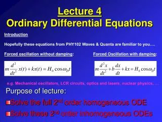
12. Exercise 1: Damped harmonic oscillator • A mass on a string is subject to a force when out of equilibrium • According to Newton’s second law (including friction), the resulting movement follows the solution to an ODE: F m y Friction Spring force Daniel Baur / Numerical Methods for Chemical Engineers / Explicit ODE Solvers

13. Assignment 1 • Rewrite the motion equation for the damped harmonic oscillator as an explicit, first order ODE system • Use ode45to solve the problem • Set up a function file to calculate the derivatives, its header should read something likefunction dy = harm_osc(t, y, m, k, a) • Set m = 1; k = 10; a = 0.5; y0 = 1; dy/dt0 = 0; • Use tSpan = [0, 20]; • Plot the position of the mass y against time • Plot the speed of the mass dy/dt against time Daniel Baur / Numerical Methods for Chemical Engineers / Explicit ODE Solvers

14. Exercise 2: Radioactive decay • A decaying radioactive element changes its concentration according to the ODEwhere k is the decay constant • The analytical solution to this problem reads Daniel Baur / Numerical Methods for Chemical Engineers / Explicit ODE Solvers

15. Assignment 2 • Plot the behavior of the radioactive decay problem as a vector field in the y vs t plane • Find online the function vector_field.m. It plots the derivatives of first order ODEs in different space and time points • Plot the vector field for y values between 0 and 1, time between 0 and 2 and k = 1. Can you see what a solver has to do? • Is it possible to switch from one trajectory in the vector field to another? What follows for the uniqueness of the solutions? • Implement the forward Euler method in a function file • The file header should read something likefunction [t,y] = eulerForward(f, t0, tend, y0, h) • Use y0 = 1, k = 1 and h = 0.1 to solve the radioactive decay problem from t0 = 0 to tEnd = 10 and plot the solution together with the analytical solution. • What happens if you increase the step size h? What happens if you increase the step size above 2? Daniel Baur / Numerical Methods for Chemical Engineers / Explicit ODE Solvers

16. Exercise 3: Lotka-Volterra equations • Predator-prey dynamics can be modeled with a simple ODE system:where x is the number of prey, y is the number of predators and a, b, c, d are parameters Daniel Baur / Numerical Methods for Chemical Engineers / Explicit ODE Solvers

17. Assignment 3 • Plot the behavior of the predator-prey system as a vector field in the x vs y plane • Find online the function vector_field2D.m which plots this vector field • Plot x and y between 0 and 1, and use a = c = 0.5 and b = d = 1 • Without solving the ODEs, what can you say about the solution behavior just by looking at the trajectories? • Solve the system using ode45, and x0 = y0 = 0.3 as initial values, and tSpan = [0, 50]; • Plot x and y against t. Can you observe what you predicted in 1? Daniel Baur / Numerical Methods for Chemical Engineers / Explicit ODE Solvers