Download
1 / 29
290 likes | 462 Views
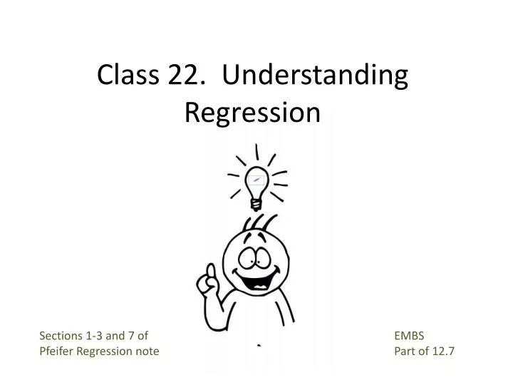
Class 22. Understanding Regression. Sections 1-3 and 7 of Pfeifer Regression note. EMBS Part of 12.7. What is the regression line?. It is a line drawn through a cloud of points. It is the line that minimizes sum of squared errors. Errors are also known as residuals.

E N D
Class 22. Understanding Regression Sections 1-3 and 7 of Pfeifer Regression note EMBS Part of 12.7
What is the regression line? • It is a line drawn through a cloud of points. • It is the line that minimizes sum of squared errors. • Errors are also known as residuals. • Error = Actual – Predicted. • Error is the vertical distance point (actual) to line (predicted). • Points above the line are positive errors. • The average of the errors will be always be zero • The regression line will always “go through” the average X, average Y. Error aka residual Predicted aka fitted
Which is the regression line? Y A B C D E F X
Which is the regression line? Y (2,7) Error = 7-3 = 4 (1,3) (2,3) (3,3) Error = 1-3 = -2 Error = 1-3 = -2 (3,1) (1,1) X Sum of Errors is 0! SSE=(-2^2+4^2+-2^2) is smaller than from any other line. The line goes through (2,3), the average.
Two Points determine a line…….and regression can give you the equation.
Two Points determine a line…….and regression can give you the equation.
Four Sets of X,Y DataData Analysis/Regression Identical Regression Output For A, B, C, and D!!!!!
Assumptions • Y is normal and we sample n independent observations. • The sample mean is the estimate of μ • The sample standard deviation s is the estimate of σ. • We use and s and n to test hypotheses about μ • Using the t-statistic and the t-distribution with n-1 dof. • We never forecasted “the next Y”. • Although, our point forecast for a new Y would be
Example: Section 4 IQs s To test H0: μ=100 n The CLT tells us this test works even if Y is not normal.
Regression Assumptions • Y│X is normal with mean a+bX and standard deviation σ, and we sample n independent observations. • We use regression to estimate a, b, and σ. • , , and “standard error” are the appropriate estimates. • Our point forecast for a new observation is + (X) • (Plug X into the regression equation) • At some point, we will learn how to use regression output to test interesting hypotheses. • What about a probability forecast of the new YlX?
EMBS (12.14) Summary: The key assumption of linear regression….. In both cases, we use the t because we don’t know σ. • Y ~ N(μ,σ) (no regression) • Y│X ~ N(a+bX,σ) (with regression) • In other words μ = a + b (X) or E(Y│X) = a + b(X) Without regression, we used data to estimate and test hypotheses about the parameter μ. With regression, we use (x,y) data to estimate and test hypotheses about the parameters a and b. The mean of Y given X is a linear function of X. With regression, we also want to use X to forecast a new Y.
Example: Assignment 22 Standard error n
Forecasting Y│X=157.3 • Plug X=157.3 into the regression equation to get 10.31 as the point forecast. • The point forecast is the mean of the probability distribution forecast. • Under Certain Assumptions……. • GOOD METHOD • Pr(Y<8) = NORMDIST(8,10.31,2.77,true) = 0.202 Assumes and and “standard error” are a, b, and σ.
Example: Assignment 22 Standard error │(X=157.3) n
Forecasting Y│X=157.3 • Plug X=157.3 into the regression equation to get 10.31 the point forecast. • The point forecast is the mean of the probability distribution forecast. • Under Certain Assumptions……. • BETTER METHOD • t= (8-10.31)/2.77 = -0.83 • Pr(Y<8) = 1-t.dist.rt(-0.83,13) = 0.210 Assumes and are a and b….but accounts for the fact that “standard error” is not σ dof = n - 2
Forecasting Y│X=157.3 • Plug X=157.3 into the regression equation to get 10.31 the point forecast. • The point forecast is the mean of the probability distribution forecast. • Under Certain Assumptions……. • PERFECT METHOD • t= (8-10.31)/2.93 = -0.79 • Pr(Y<8) = 1-t.dist.rt(-0.79,13) = 0.222 To account for using and to estimate a and b, we must increase the standard deviation used in the forecast. The “correct” standard deviation is called “standard error of prediction”…which here is 0.293. dof = n - 2
Probability Forecasting with Regressionsummary • Plug X into the regression equation to calculate the point forecast. • This becomes the mean. • GOOD • Use the normal with “standard error” in place of σ. • BETTER • Use the t (with n-2 dof) to account for using “standard error” to estimate σ. • PERFECT • Use the t with the “standard error of prediction” to account for using and to estimate a and b.
Probability Forecasting with Regression • “Standard error of prediction” is larger than “standard error” and depends on • 1/n (the larger the n the smaller is “standard error of prediction”) • (X-)^2 (the farther the X is from the average X, the larger is “standard error of prediction”) • As n gets big, the “standard error of prediction” approaches “standard error”.
(EMBS 12.26) The X for which we predict Y The good and better methods ignore these terms…okay the bigger the n. Summed over the n data points
BOTTOM LINE • You will be asked to use the BETTER METHOD • Use the t with n-2 dof • Just use “standard error” • Know that “standard error” is smaller than the correct “standard deviation of prediction”. • As a result, your probability distribution is a little too narrow. • Know that the “standard deviation of prediction” depends on 1/n and (X-)^2 … which means it approaches “standard error” as n gets big.
Much ado about nothing? Perfect (widest and curved) Better Good (straight and narrowest)
TODAY • Got a better idea of how the “least squares” regression line goes through the cloud of points. • Saw that several “clouds” can have exactly the same regression line….so chart the cloud. • Practiced using a regression equation to calculate a point forecast (a mean) • Saw three methods for creating a probability distribution forecast of Y│X. • We will use the better method. • We will know that it understates the actual uncertainty…..a problem that goes away as n gets big.
Next Class • We will learn about “adjusted R square” • (p 9-10 pfeifer note) • The most over-rated statistic of all time. • We will learn the four assumptions required to use regression to make a probability forecast of Y│X. • (Section 5 pfeifer note, 12.4 EMBS) • And how to check each of them. • We will learn how to test H0: b=0. • (p 12-13 pfeifer note, 12.5 EMBS) • And why this is such an important test.