Download

1 / 24
240 likes | 389 Views
ZGOUBI application to NS-FFAG. Takeichiro Yokoi (JAI). BD. BF1. BF2. 15º. 15º. R 0. Why ZGOUBI ?. (1) Idealized model, 3D tracking are treated in the same framework (2) Well-fit to wide orbit excursion accelerator such as FFAG

E N D
ZGOUBI application to NS-FFAG Takeichiro Yokoi (JAI)
BD BF1 BF2 15º 15º R0 Why ZGOUBI ? (1) Idealized model, 3D tracking are treated in the same framework (2) Well-fit to wide orbit excursion accelerator such as FFAG (3) Global coordinate lattice is easily built. (especially helps for PAMELA) (4) Beam acceleration is implemented DIPOLE geometry Geometry of PAMELA (co-centric lattice)
Magnet center A B A B C D D C QD QF 3D field tracking Why 3D tracking ? Field coupling between BF and BD is non-linear Fringing field is major part in a thin magnet (3) Field distribution is not that of ideal quadrupole (especially in outer region) **Fields are calculated with OPERA/3D
Field superposition Field distribution of cell can be expressed with a superposition of individual magnet( with a precision of less than 0.2%) No vertical dependence Sum(QF+QD) Inter-magnet region Sum(QF+QD) Sum(QF+QD)-Cell
Scalability check of single magnet For a confirmation, field scalability of QD among different current settings was checked. The same setup as page 2 was used (Current of QF is set zero.) X(cm) X(cm) By(I=500A) By(I=500A)-500/201.3*By(I=200A) Within the plausible current range, the field scalability of QD is confirmed. Maximum difference is less than 0.1%
Chamfer: 0mm ∆By(gauss) Magnet pole Chamfer: 1mm Chamfer: 2mm Chamfer: 4mm Z(cm) Effect of chamfer for QF Looking from this direction By(I=400A)-400/201.5*By(I=200A) For QF, weak edge saturation is observed For safety, it might be better to employ chamfer of ~2mm
386mm 8.48mm ±65mm Y X 8.5714˚ 8.5714˚ 104mm 104.76mm Map geometry Drift space for adjustment Field map Mesh size X: 1mm,Y: 1mm, Z: 1mm (rough optimization was carried out)
Procedure for coil current optimization • Scan coil-current coarsely to find a current set of symmetric path length for each lattice. (nominal current: I0(QD) I0(QF) ) • Adjust I(QD), I(QF) around I0(QD) and I0(QF) keeping symmetry of path length so that the tunes are close to the design value. • (Tweak the magnet shape) then iterate step 1~3
Comparison with baseline lattice Baseline Tracking ** Field map was generated for individual operating point • Low energy region(<12MeV) shows larger discrepancy
QF QD + 2.0cm Parameterization of current As a nominal focusing power, focusing power of region 2 was taken
baseline tracking 70221f 70221b 70221g 70221h 70221e 70221c 70221i 70221d Comparison with baseline lattice Due to the inter-magnet coupling, effective focusing power gets reduced compared to that of the baseline model (10~15%)
Dynamic Aperture Survey 12MeV 10MeV 15MeV 18MeV 20MeV 70221c
The difficulty of injection in EMMA FFAG is to cope with the broader varieties of injection conditions (Energy:10MeV~20MeV, tune: ~0.1~0.4> /cell, various operational modes) • With the 2-kicker scheme, beam position in the phase space can be tuned with some degree of flexibility • Actually,with optimization, how large is the distribution?
Setup QD1 QF1 QD2 QD0 QF2 QF0 Beam Septum Kicker Kicker Beam position was monitored at the center of each magnet and short straight section
Tracking study(2kicker option) 061209c Septum boundary For the realistic extraction scheme, beam distribution over entire operating point should be minimized 10MeV +0.45kgauss -0.45kgauss Kicked beam@septum Kicked beam @mid of 2nd kicker 15MeV Circulating beam 0.0kgauss -0.55kgauss 20MeV 0.0kgauss -0.5kgauss
Beam distribution at septum (extraction) With 3D map 40mrad. 70221b 2mm Septum septum
Required GFR(±32mm) Required GFR(±56mm) 70221b 70221b QF1 QD1 70221c 70221c 70221d 70221d Xmax Xmin 70221b 70221b QD2 70221c QF2 70221c 70221d 70221d Center of magnet Beam envelope in magnet (extraction)
Beam distribution at septum (extraction) With MULTIPOL ∆x’:40mrad 70221b ∆x:2.5mm At least, injection and extraction, 3D field tracking is indispensable
Working Environment In real simulation study, unified working environment including (1) preprocessing (2) job control (3) post processing(+ online automatic analysis) (4) external function call(unix shell) is desirable. Ex. tune survey of EMMA typical number of input file >40. error study in PAMELA., typical run>50, each run>3hour. Online analysis is the key issue for mass processing. (Actually, ZPOP is a hardwired program and not flexible.)
Input file generation “zgoubi.dat” etc PAW Run “ZGOUBI” “zgoubi.plt” , “zgoubi.fai” Analysis Data-Summary Working Environment For working environment, PAW developed by CERN is employed. Function of PAW: plotting, analysis(ex ntuple), script language, external function call • Problems : Obsolete (no more maintained by CERN) • Numerical bugs in script environment (not frequent) • Now, ROOT** based environment is developing ** C++ based unified analysis tool
User function call External function call Analysis Example of PAW macro ( for automatic CO+ optical parameter calculation)