Download
1 / 20
200 likes | 213 Views
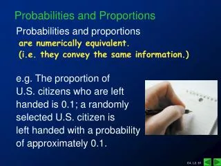
Explore random experiments, sample spaces, permutations, combinations, and equi-probable spaces in probability theory. Learn to quantify uncertainty and analyze outcomes.

E N D
15 Chances, Probabilities, and Odds 15.1 Random Experiments and Sample Spaces 15.2 Counting Outcomes in Sample Spaces 15.3 Permutations and Combinations 15.4 Probability Spaces 15.5 Equiprobable Spaces 15.6 Odds
Random Experiment In broad terms, probability is the quantification of uncertainty. To understandwhat that means, we may start by formalizing the notion of uncertainty. We will use the term random experiment to describe an activity or a processwhose outcome cannot be predicted ahead of time. Typical examples of randomexperiments are tossing a coin, rolling a pair of dice, drawing cards out of a deckof cards, predicting the result of a football game, and forecasting the path of ahurricane.
Sample Space Associated with every random experiment is the set of all of its possible outcomes, called the sample space of the experiment. For the sake of simplicity, wewill concentrate on experiments for which there is only a finite set of outcomes,although experiments with infinitely many outcomes are both possible and important.
Sample Space - Set Notation Since the sample space of any experiment is a set of outcomes, we will useset notation to describe it. We will consistently use the letter S to denote a samplespace and the letter N to denote the size of the sample space S (i.e., the numberof outcomes in S).
Example 15.1 Tossing a Coin One simple random experiment is to toss a quarter and observe whether it lands heads or tails. The sample space can be described by S = {H, T},where H standsfor Heads and T for Tails. Here N = 2.
Example 15.2 More Coin Tossing Suppose we toss a coin twice and record the outcome of each toss (H or T) in theorder it happens. The sample space now isS = {HH, HT, TH, TT},where HTmeans that the first toss came up H and the second toss came up T, which is adifferent outcome from TH (first toss T and second toss H). In this sample space N = 4.
Example 15.2 More Coin Tossing Suppose now we toss two distinguishable coins (say, a nickel and a quarter)at the same time (tricky but definitely possible). This random experiment appears different from the one where we toss one coin twice, but the sample spaceis stillS = {HH, HT, TH, TT}. (Here we must agree what the order of thesymbols is–for example, the first symbol describes the quarter and the secondthe nickel.)
Example 15.2 More Coin Tossing Since they have the same sample space, we will consider the two random experiments just described as the same random experiment.Now let’s consider a different random experiment. We are still tossing a cointwice, but we only care now about the number of heads that come up. Here thereare only three possible outcomes (no heads, one head, or both heads), and symbolically we might describe this sample space asS = {0, 1, 2}.
Example 15.3 Shooting Free Throws Here is a familiar scenario: Your favorite basketball team is down by 1, clock running out, and one of your players is fouled and goes to the line to shoot freethrows, with the game riding on the outcome. It’s not a good time to think of sample spaces, but let’s do it anyway.Clearly the shooting of free throws is a random experiment, but what is thesample space? As in Example 15.2, the answer depends on a few subtleties.
Example 15.3 Shooting Free Throws In one scenario (the penalty situation) your player is going to shoot two freethrows no matter what. In this case one could argue that what really matters ishow many free throws he or she makes (make both and win the game, miss oneand tie and go to overtime, miss both and lose the game). When we look at it thisway the sample space isS = {0, 1, 2}.
Example 15.3 Shooting Free Throws A somewhat more stressful scenario is when your player is shooting a one-and-one. This means that the player gets to shoot the second free throw only if heor she makes the first one. In this case there are also three possible outcomes, butthe circumstances are different because the order of events is relevant (miss thefirst free throw and lose the game, make the first free throw but miss the secondone and tie the game, make both and win the game).
Example 15.3 Shooting Free Throws We can describe this samplespace asS = {ff, sf, ss},where we use f to indicate failure (missed the freethrow) and s to indicate success.
Example 15.4 Rolling a Pair of Dice The most common scenario when rolling a pair of dice is to only consider thetotal of the two numbers rolled. In this situation we don’t really care how a particular total comes about. We can “roll a seven” in various paired combinations–a3 and a 4, a 2 and a 5, a 1 and a 6. No matter how the individual dice come up, theonly thing that matters is the total rolled.
Example 15.4 Rolling a Pair of Dice The possible outcomes in this scenario range from “rolling a two” to “rollinga twelve,” and the sample space can be described byS = {2, 3, 4, 5, 6, 7, 8, 9,10,11,12}.
Example 15.5 More Dice Rolling A more general scenario when rolling a pair of dice is when we do care whatnumber each individual die turns up (in certain bets in craps, for example, two “fours” is a winner but a “five” and a “three” is not). Here wehave a sample space with 36 different outcomes.
Example 15.5 More Dice Rolling Notice that the dice are colored white andred, a symbolic way to emphasize the fact that we are treating the dice as distinguishable objects. That is why the rolls and are considered different outcomes.
Example 15.6 More Dice Rolling Five candidates (A, B, C, D, and E) are running in an election. The top three votegetters are chosen President, Vice President, and Secretary, in that order. Such anelection can be considered a random experiment with sample space S = {ABC,ACB, BAC, BCA, CAB, CBA, ABD, ADB,…, CDE}.We will assume thatoutcome ABC denotes that candidate A is elected President, B is elected Vice President, and C is elected Secretary.
Example 15.6 More Dice Rolling This is important because the outcomes ABC andBAC are different outcomes and must appear separately in the sample space. Because this sample space is a bit too large to write out in full (we will soonlearn that its size is N = 60), we use the “. . .” notation. It is a way of saying “andso on–you get the point.”
Not Listing All of the Outcomes Example 15.6 illustrates the point that sample spaces can have a lot of outcomes and that we are often justified in not writing each and every one of themdown. This is where the “. . .” comes in handy. The key thing is to understand whatthe sample space looks like without necessarily writing all the outcomes down.Our real goal is to find N, the size of the sample space. If we can do it withouthaving to list all the outcomes, then so much the better.