Download
1 / 84
850 likes | 889 Views
Learn about quantum distribution functions for bosons, fermions, and other objects, with detailed balance principles and applications of the Lagrange multiplier technique in this formalism outline. The text covers Boltzmann distribution functions, probabilities for particles, and detailed balance for distinguishable and indistinguishable particles.

E N D
Quantum Distribution FunctionsforBosons, Fermions, & otherwise Objects Formalism: Appendix C Ch 11.1-11.4 Applications: Ch 11.5-11.11 http://www.slimy.com/~steuard/teaching/tutorials/Lagrange.html http://www.cs.berkeley.edu/~klein/papers/lagrange-multipliers.pdf
FORMALISM OUTLINE • Quick Basic Probability Ideas • Boltzmann Distribution Fn: App C • Comparison of Ytot* Ytot for Bosons & Fermions: 11-2 • Detailed Balance: 11-3 • w/o special requirements • bosons • fermions • Distribution Fns: 11-4 • various interpretations of the ea factor
How to do the Lagrange Multiplier technique • function f(x1, x2, …) • Constraint g(x1, x2, …)=c • Form new function F = f + l (g-c) • Maximize it wrt x1, x2, … • Choose something for l based upon other information Maximize a function subject to certain constraints on the dependent variables
Example Maximize f = xy subject to constraint x2+y2=1 F = xy +l (x2+y2-1) dF/dx = y + 2lx = 0 -2l = y/x y/x = x/y x2 = y2 dF/dy = x + 2ly = 0 -2l = x/y x2+y2=1 x2+x2=1 2x2 = 1 x=0.707
Example Minimize f = xy subject to constraint x2+y2=1 F = xy +l (x2+y2-1) (y+2lx) + (x+2ly) = 0 dF/dx = y + 2lx (1+2l)y + (1+2l)x = 0 dF/dy = x + 2ly y = -x x2+y2=1 x2+x2=1 2x2 = 1 x=±0.707
Given N=5 objects and p=1 bin; How many ways can one put n=2 objects in the bin ? (in a definite order)
Given N=5 objects and p=1 bin; How many ways can one put n=2 objects in the bin ? (without regard to order) Note that after filling this box, there are (N-n) objects unused.
Given N total objects and p total bins; How many ways can one put n1 objects in bin #1 n2 objects in bin #2 n3 objects in bin #3 * * * (without regard to order) * * *
* * * n1 n2 n3
Probability Summary N total objects p total states np * * * n5 n4 n3 n2 n1
BOLTZMANN DISTRIBUTION Probability of finding a particular energy e subject to the constraint that there are N total particles and Etot energy
p * * * 2 1
p * * * 2 1
Sterling’s Formula The second term is largest by at least a parsec
To discover the expression for the normalization constant OK, so what is b = ?
Temperature is defined in terms of the average kinetic energy
Boltzmann Distribution Probability of finding a particular energy e subject to the constraints that there are N total particles and fixed Etot ea = 1/kT
Many, many closely-spaced states,but with restriction on filling
11-2 COMPARING PROBABILITIES Y*Yfor Indistinguishable Boson/Fermion Particles to thosewithout worrying about B/F requirements OR what do the B/F requirements do to probabilities?
Distinguishable Particle Probabilities One particle in a state b Ytot = Yb(1) Prob = Ytot* Ytot = Yb(1) *Yb(1) = 1 Two particles in a state b Ytot = Yb(1) Yb(2) Prob = Yb(1)*Yb(1) Yb(2)*Yb(2) = 1 Three particles in a state b Ytot = Yb(1) Yb(2) Yb(3) Prob = Yb(1)*Yb(1) Yb(2)*Yb(2) Yb(3)*Yb(3) = 1 So what ? Nothing special happens here…..
Indistinguishable Boson Probabilities One particle in a state b Ytot = Yb(1) Prob = Ytot* Ytot = Yb(1) *Yb(1) = 1 Two particles in a state b Ytot = [Yb(1) Yb(2) + Yb(2) Yb(1)] = 2 Yb(1) Yb(2) Prob = | 2 Yb(1) Yb(2) |2 = 2 = 2! Three particles in a state b Ytot = [ Yb(1) Yb(2) Yb(3) + … ] Prob = | 6 Yb(1) Yb(2) Yb(3) |2 = 6 = 3! If there are already n bosons in a state, the probability of one more joining them is enhanced by (1+n) than what the prob would be w/o indistinguishability requirements
Indistinguishable Fermion Probabilities One particle in a state b Ytot = Yb(1) Prob = Ytot* Ytot = Yb(1) *Yb(1) = 1 Two particles in a state b Ytot = [Yb(1) Yb(2) - Yb(2) Yb(1)] = 0 Prob = 0 If there are already n fermions in a state, the probability of one more joining them is enhanced by (1-n) than what the prob would be w/o indistinguishability requirements
Principle of Detailed Balance For two states of a system with fixed total energy, n2 e2 n1 e1 Where the particles can jump between states by some unknown mechanism, Rate of upward going transitions = Rate of downward going transitions n1 Rate 12 = n2 Rate 21 transitions/sec per particle
Detailed Balance distinguishable particles(but with no other special requirements) Since by the Boltzmann distribution n ~ e-e/kT Gives us the ratio of the two transition rates
Bose distribution function Probable # bosons of an energy e in a system of fixed total energy at a temperature T
Detailed Balance indistinguishable fermions ( short derivation )
Fermi distribution function Probable # fermions of an energy e in a system of fixed total energy at a temperature T
Normalization Interpretation * * This interpretation may not be so useful for Bose & Fermi distributions * For Ntot free particles strictly confined to a 3-D region of space of volume V.
Chemical Potential Interpretation m = - a kT A uniform description for all three distributions. Used for Bose distribution.