Download
1 / 41
410 likes | 537 Views
Statistical Postprocessing of Weather Parameters for a High-Resolution Limited-Area Model. Susanne Theis Andreas Hense. Ulrich Damrath Volker Renner. Overview. - Introduction - Description of Method - Examples - Verification Results - Calibration of Reliability Diagrams

E N D
Statistical Postprocessing of Weather Parameters for a High-Resolution Limited-Area Model Susanne Theis Andreas Hense Ulrich Damrath Volker Renner
Overview - Introduction - Description of Method - Examples - Verification Results - Calibration of Reliability Diagrams - Concluding Remarks
Basic Set-up of the LM • Model Configuration • Full DM model domain with a grid • spacing of 0.0625o (~ 7 km) • 325 x 325 grid points per layer • 35 vertical layers • timestep: 40 s • three daily runs at 00, 12, 18 UTC • Boundary Conditions • Interpolated GME-forecasts with • ds ~ 60 km and 31 layers (hourly) • Hydrostatic pressure at lateral • boundaries • Data Assimilation • Nudging analysis scheme • Variational soil moisture analysis • SST analysis 00 UTC • Snow depth analysis every 6 h Deutscher Wetterdienst
LM Total Precipitation [mm/h] 08.Sept.2001, 00 UTC, vv=14-15 h
Methods - Neighbourhood Method (NM) - Wavelet Method - Experimental Ensemble Integrations
Neighbourhood Method Assumption: LM-forecasts within a spatio-temporal neighbourhood are assumed to constitute a sample of the forecast at the central grid point
x x Definition of Neighbourhood I y t
Definition of Neighbourhood II Size of Area Form of Area hs Linear Regressions
Definition of the Quantile Function The quantile function x is a function of probability p. If the forecast is distributed according to the probability distribution function F, then x(p) := F-1(p) for all p [0, 1]. There is a probability p that the quantile x(p) is greater than the correct forecast. (Method according to Moon & Lall, 1994)
Products • „Statistically smoothed” fields • Quantiles for p = 0.5 • Expectation Values • Probabilistic Information • Quantiles • (Probabilities for certain threshold values)
LM Total Precipitation [mm/h] 08.Sept.2001, 00 UTC, vv=14-15 h Original Forecast Expectation Values
LM Total Precipitation [mm/h] 08.Sept.2001, 00 UTC, vv=14-15 h Original Forecast Quantiles for p=0.9
LM T2m [oC] 08.Sept.2001, 00 UTC, vv=15 h Original Forecast Quantiles for p=0.5
Direct model output of the LM for precipitation at a given grid point
...supplemented by more quantiles (forecast of uncertainty)
...supplemented by the 90 %-quantile (forecast of risk)
Verification Data LM forecasts; 1.-15.09.2001; 00 UTC starting time 1 h values; 6-30 h forecast time all SYNOPs available from German stations comparison with nearest land grid point NM-Versions small: 3 time levels (3 h); radius: 3s ( 20 km) medium: 3 time levels (3 h); radius: 5s ( 35 km) large: 7 time levels (7 h); radius: 7s ( 50 km) Averaging square areas of different sizes temperatures adjusted with -0.65 K/(100 m)
Richardson, D.S., 2001: Measures of skill and value of ensemble prediction systems, their interrelationship and the effect of ensemble size. Q.J.R.Meteorol.Soc., Vol.127, pp. 2473-2489)
Calibration • Empirical Approach: • use a large data sets of forecasts and observations • PRO: covers all relevant effects • CON: calibration is dependent on LM-version • Theoretical Approach: • focus on the effect of limited sample size only • PRO: effect can be quantified theoretically, without large data sets • calibration is independent of LM-version • CON: all other effects are neglected
Calibration Procedure: • choose probability p of the desired quantile • (e.g. p=90%, if you would like to estimate the 90%-quantile) • determine sample size M, frequency m of the event and • predictability s of the event (a priori) • calculate a probability p' = p' (p,M,m,s) from statistical • theory (Richardson, 2001), let‘s say p' = 95% • estimate 95%-quantile and redefine it as a 90%-quantile
p p' Richardson, D.S., 2001: Measures of skill and value of ensemble prediction systems, their interrelationship and the effect of ensemble size. Q.J.R.Meteorol.Soc., Vol.127, pp. 2473-2489)
Preliminary Results of Calibration (small neighbourhood): (LM forecasts; 10.-24.07.2002; 00 UTC starting time) Determination of p' = p' (p,M,m,s) : integrate p' = p' (p,M,m,s) over all possible values of m and sand over M=[1,80]
Effect of Limited Sample Size on Quantiles for p=0.9 Probability of exceedance of depending on the observed frequency μ for different values of effective sample size M and a prescribed value of σ2=0.25 m (1-m)
Concluding Remarks “Statistically Smoothed” Fields For temperature no mean advantage is to be seen in comparison with simple averaging The results for precipitation are difficult to judge upon; proper choice amongst the various possibilities is still an open question Reliability Diagrams Possible improvement by calibration remains to be explored The results for precipitation clearly demonstrate the need for improving the model (reduce the overforecasting of slight precipitation amounts)
Concluding Remarks (ctd.) Application The method might be useful not only for single forecasts but also in combination with small ensembles