Download
1 / 70
700 likes | 853 Views
Face detection with boosted Gaussian features. Pattern Recognition, Feb, 2007 井民全 報告. Outline. Introduction A brief overview of AdaBoost The VC-Dimension concept The features Anisotropic Gaussian filters Gaussian vs. Haar-like Experiments and results. Introduction.

E N D
Face detection with boosted Gaussian features Pattern Recognition, Feb, 2007 井民全 報告
Outline • Introduction • A brief overview of AdaBoost • The VC-Dimension concept • The features • Anisotropic Gaussian filters • Gaussian vs. Haar-like • Experiments and results
Introduction • Automatic face detection is a key step in any face processing system • It is far from a trivial task • faces are highly deformable objects • lighting conditions, poses • holistic methods • consider the face as a global object • feature-based methods • recognize parts of the face and assemble them to take the final decision
Introduction • The classical approach for face detection Step 1: scan the input image with a sliding window, and for each position Step 2: the window is classified as either face or non-face • The efficient exploration of the search space is a key ingredient for obtaining a fast face detector • Skin color, a coarse-to-fine approach, etc…
Introduction • A fast algorithm is proposed by Viola and Jones • Three main ideas • first train a strong classifier by Haar-like features-based classifiers • use the so-called integral image as image representation very efficiently • a classification structure in cascade speed
A brief overview of AdaBoost 24 a strong classifier 24 h1 h2 h3 h4 hT-1 hT Weaker classifier
Stage 3 Stage 2 Pass Pass Ada Boosting Learner Ada Boosting Learner False (Reject) False (Reject) Cascaded Classifiers Structure Stage 1 Feature set Ada Boosting Learner Feature Select & Classifier 100% Detection Rate 50% False Positive False (Reject) Reject as many negatives as possible (minimize the false negative)
The region have the same size and shape And are horizontally or vertically adjacent Three-Rectangle Feature the sum within two outside rectangle subtracted from the sum in a center rectangle Four-Rectangle Feature The difference between the diagonal pairs of rectangles The base resolution is 24x24 The exhaustive set of rectangle is large, over 180,000. Haar-like features The difference between the sum of pixels within two rectangular regions 1 Two-Rectangle Feature 2 3
The feature values An example 24 24 Over 180,000 rectangle features associate with each sub-image
The training process for a weaker learner • Let’s see an example
The training process for a weaker classifier (an example) Example xi Example x yi y {f1(x),f2(x),…,fj(x), …, f180,000(x)} 1 {10,23,…,5, …} h1 {7,20,…, 25, …} 1 h1(xi)= 1 , if fj(xi) < 30 0, otherwise 0 {15,21,…,100,…} Searching for a feature that the training error is minimal ! {15,21,…,20,…} 0 fj(x)
The 1st iteration Example xi Example x y yi fj(x) h1(x) 1 {10,23,…,5, …} 1 h1 {7,20,…, 25, …} 1 1 h1(xi)= 1 , if fj(xi) < 30 0, otherwise 0 0 {15,21,…,100,…} {7,23,…,20,…} 1 (False positive) 0
h1 h1(xi)= 1 , if fj(xi) < 30 0, otherwise False positive Non-face
The training error for h1 Example xi yi fj(x) h1(x) weight error 1 {10,23,…,5, …} 1 1/4 0 + {7,20,…, 25, …} 1 1/4 0 1 + = 1/4 for h1 0 1/4 0 0 {15,21,…,100,…} + {7,23,…, 20,…} (False positive) 1 1/4 1/4 0
Update the weight (1/2) Distribute the contribution!
Update the weight (2/2) Example xi yi fj(x) h1(x) Weight error 1 {10,23,…,5, …} 1 1/4* 0 (變小) + {7,20,…, 25, …} 1/4* 1 0 1 (變小) + = 1/4 for h1 0 0 0 {15,21,…,100,…} 1/4* (變小) + {7,23,…, 20,…} (False positive) 1 1/4 1/4 0 (不變)
Normalization the weight N= # of the example
Normalize Weight Example xi yi fj(x) h1(x) 1 {10,23,…,5, …} 1 0.166 {7,20,…, 25, …} 0.166 1 1 0 0 {15,21,…,100,…} 0.166 {7,23,…, 20,…} (False positive) 1 0.5 0 (剛剛分錯的, weight 變大 由 1/4 0.5)
分析 目前 使用 feature j 進行分類, 整體的 training error • 因為我們選 classifier 是選擇產生總體分類錯誤最小的 feature , 進行分類. • 而上次的分類, 分錯的 example 錯誤成本增加了. 故整個 training process 會趨向不讓上次分錯的 example, 在這次分錯 每一個 example 的 weight (錯誤成本)
Cascaded Classifiers Structure h1 h2 False positive of h1 Non-face
Step 1: Giving example images Image The Boost algorithm for classifier learning Positive =1 Negative=0 Step 2: Initialize the weights For t = 1, … , T 1. Normalize the weights, 2. For each feature j, train a classifier hj which is restricted to using a single feature 3. Update the weights: Weak learner constructor
The final strong classifier 若超過一半的人, 贊成就通過 每個人的投票的份量, 由正確率決定
Introduction • A brief overview of AdaBoost • The VC-Dimension concept • The features • Anisotropic Gaussian filters • Gaussian vs. Haar-like • Experiments and results
The VC-Dimension concept • A learning machine f takes an input x and transforms it, somehow using weights a, into a predicted output in some pagers, the definition is (Some vector of adjustable parameters) f
Examples f
Examples f
Examples f
How do we characterize “power”? • Different machines have different amounts of “power” • Tradeoff between: • More power: Can model more complex classifiers but might overfit • Less power: Not going to overfit, but restricted in what it can model • How do we characterize the amount of power?
Some definitions • Given some machine f • And under the assumption that all training points (xk,yk) were drawn i.i.d from some distribution. • And under the assumption that future test points will be drawn from the same distribution i.i.d independent and identically distributed
Probability of misclassification Fraction training set of misclassification 片段 R = # of training
known Vapnik-Chervonenkis dimension • Given some machine f, let h be its VC dimension • Vapnik showed that Known(# of training example) with probability 1-
known known This gives us a way to estimate the error on future data based only on the training error and the VC-dimension of f
But given machine f, how do we define and compute h? the VC-dimension of f
Shattering • Machine f can shatter a set of points x1, x2 .. xr if and only if… • For every possible training set of the form • There exists some value of that gets zero training error.
Question • Can the following f shatter the following points?
Answer: No problem • There are four training sets to consider 水平線 (ok) 對角線 (ok) 對角線換正負號 (ok) 水平線換正負號 (ok)
Question • Can the following f shatter the following points?
Answer: No way my friend 衝突 無法變換參數 (因為 f(x,b) 中無法控制 x 圓外一類 圓內一類 (ok) 圓外一類 圓內一類 (ok)
Definition of VC dimension • Given machine f, the VC-dimension h is The maximum number of points that can be arranged so that f shatter them 這個機器, 在所有 example 組合下, 最多不會分錯的 example 個數 • What ‘s VC dimension of Ans: 1
VC dim of line machine • For 2-d inputs, what’s VC-dim of f(x,w,b) = sign(w.x+b)? • Well, can we find four points that f can shatter? …
Structural Risk Minimization • considers a sequence of hypothesis spaces of increasing complexity • For example, polynomials of increasing degree.
Structural Risk Minimization • We’re trying to decide which machine to use • We train each machine and make a table… 越簡單 越複雜
分析 • Vapnic-Chervonenkis 告訴我們任一台機器的 TestError 與 VC-Dimension (機器複雜程度) 有關. • 對相同 data set 而言, 複雜度越高的機器, 對 training 資料 overfit 的程度也越高. Training example
Generalization error for the AdaBoost proposed by Freund d= VC-dimension TRAINERR
For example • An AdaBoost algorithm proposed by [1] • Total # of features in all layer 6061 • AdaBoost has an important drawback • It tends to overfit training examples
Introduction • A brief overview of AdaBoost • The VC-Dimension concept • The features • Anisotropic Gaussian filters • Gaussian vs. Haar-like • Experiments and results
The proposed new features – Anisotropic Gaussianfilters • The generating function • It efficiently capture contour singularities with a smooth low resolution function
The transformations • Translation by • Rotation by • Bending by r
Anisotropic scaling by • By combining these four basic transforations,