Download
1 / 23
230 likes | 251 Views
Explore advanced copula modeling methods for simulating joint probabilities and handling tail behavior. Learn about popular copula families such as Frank's, Gumbel, and Normal copulas, along with tailored parameterization approaches. Gain insights into heavy-tailed copulas and pairwise concept distributions in this comprehensive guide.

E N D
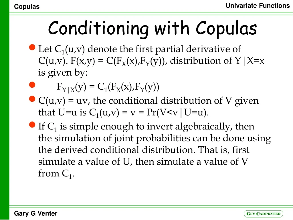
Conditioningwith Copulas • Let C1(u,v) denote the first partial derivative of C(u,v). F(x,y) = C(FX(x),FY(y)), distribution of Y|X=x is given by: • FY|X(y) = C1(FX(x),FY(y)) • C(u,v) = uv, the conditional distribution of V given that U=u is C1(u,v) = v = Pr(V<v|U=u). • If C1 is simple enough to invert algebraically, then the simulation of joint probabilities can be done using the derived conditional distribution. That is, first simulate a value of U, then simulate a value of V from C1.
Tails of Copulas ASTIN 2001
Kendall correlation • t is a constant of the copula • t = 4E[C(u,v)] – 1 • t = 2dE[C(u1, . . .,ud)] – 1 2d – 1 – 1
Frank’s Copula • Define gz = e-az – 1 • Frank’s copula with parameter a 0 can be expressed as: • C(u,v) = -a-1ln[1 + gugv/g1] • C1(u,v) = [gugv+gv]/[gugv+g1] • c(u,v) = -ag1(1+gu+v)/(gugv+g1)2 • t(a) = 1 – 4/a + 4/a20a t/(et-1) dt • For a<0 this will give negative values of t. • v = C1-1(p|u) = -a-1ln{1+pg1/[1+gu(1–p)]}
Gumbel Copula • C(u,v) = exp{- [(- ln u)a + (- ln v)a]1/a}, a 1. • C1(u,v) = C(u,v)[(- ln u)a + (- ln v)a]-1+1/a(-ln u)a-1/u • c(u,v) = C(u,v)u-1v-1[(-ln u)a +(-ln v)a]-2+2/a[(ln u)(ln v)]a-1 {1+(a-1)[(-ln u)a +(-ln v)a]-1/a} • t(a) = 1 – 1/a • Simulate two independent uniform deviates u and v • Solve numerically for s>0 with ues = 1 + as • The pair [exp(-sva), exp(-s(1-v)a)] will have the Gumbel copula distribution
Heavy Right Tail Copula • C(u,v) = u + v – 1 + [(1 – u)-1/a + (1 – v)-1/a – 1]-a a>0 • C1(u,v) = 1 – [(1 – u)-1/a + (1 – v)-1/a – 1] -a-1(1 – u)-1-1/a • c(u,v) = (1+1/a)[(1–u)-1/a +(1– v)-1/a –1] -a-2[(1–u)(1–v)]-1-1/a • t(a) = 1/(2a + 1) • Can solve conditional distribution for v
Joint Burr • F(x) = 1 – (1 + (x/b)p)-a and G(y) = 1 – (1 + (y/d)q)-a • F(x,y) = 1 – (1 + (x/b)p)-a – (1 + (y/d)q)-a + [1 + (x/b)p + (y/d)q]-a • The conditional distribution of y|X=x is also Burr: • FY|X(y|x) = 1 – [1 + (y/dx)q]-(a+1), where dx =d[1 + (x/b)p/q]
Partial Perfect Correlation Copula Generator • Assume logical values 0 and 1 are arithmetic also • h : unit square unit interval • H(x) = 0xh(t)dt • C(u,v) = uv – H(u)H(v) + H(1)H(min(u,v)) • C1(u,v) = v – h(u)H(v) + H(1)h(u)(v>u) • c(u,v) = 1 – h(u)h(v) + H(1)h(u)(u=v)
h(u) = (u>a) • H(u) = (u – a)(u>a) • t(a) = (1 – a)4
h(u) = ua • H(u) = ua+1/(a+1) • t(a) = 1/[3(a+1)4] + 8/[(a+1)(a+2)2(a+3)]
The Normal Copula • N(x) = N(x;0,1) • B(x,y;a) = bivariate normal distribution function, = a • Let p(u) be the percentile function for the standard normal: • N(p(u)) = u, dN(p(u))/du = N’(p(u))p’(u) = 1 • C(u,v) = B(p(u),p(v);a) • C1(u,v) = N(p(v);ap(u),1-a2) • c(u,v) = 1/{(1-a2)0.5exp([a2p(u)2-2ap(u)p(v)+a2p(v)2]/[2(1-a2)])} • t(a) = 2arcsin(a)/p • a: 0.15643 0.38268 0.70711 0.92388 0.98769 • t: 0.10000 0.25000 0.50000 0.75000 0.90000
Tail Concentration Functions • L(z) = Pr(U<z,V<z)/z2 • R(z) = Pr(U>z,V>z)/(1 – z)2 • L(z) = C(z,z)/z2 • 1 - Pr(U>z,V>z) = Pr(U<z) + Pr(V<z) - Pr(U<z,V<z) • = z + z – C(z,z). • Then R(z) = [1 – 2z +C(z,z)]/(1 – z)2 • Generalizes to multi-variate case
Cumulative Tau • t = –1+40101 C(u,v)c(u,v)dvdu • J(z) = –1+40z0z C(u,v)c(u,v)dvdu/C(z,z)2 • Generalizes to multi-variate case
Cumulative Conditional Mean • M(z) = E(V|U<z) = z-10z01 vc(u,v)dvdu • M(1) = ½ • A pairwise concept Copula Distribution Function • K(z) = Pr(C(u,v)<z) • Generalizes to multi-variate case
HRT Gumbel Frank Normal Parameter 0.968 1.67 4.92 0.624 Ln Likelihood 124 157 183 176 Tau 0.34 0.40 0.45 0.43