Download
1 / 36
360 likes | 543 Views
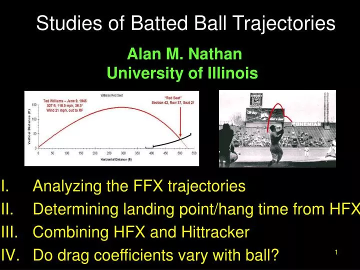
Studies of Batted Ball Trajectories. Alan M. Nathan University of Illinois. I. Analyzing the FFX trajectories II. Determining landing point/hang time from HFX Combining HFX and Hittracker Do drag coefficients vary with ball?. I. Analyzing FFX Trajectories. WWAD = What Would Alan Do?

E N D
Studies of Batted Ball Trajectories Alan M. Nathan University of Illinois I. Analyzing the FFX trajectories II. Determining landing point/hang time from HFX • Combining HFX and Hittracker • Do drag coefficients vary with ball? Nathan, Summit2010
I. Analyzing FFX Trajectories • WWAD = What Would Alan Do? • Actually, what DID Alan do? • Scottsdale, March 2009 experiment • 10 Cameras uses • 2 PFX/HFX cameras • 8 IP cameras • *All* data used to analyze trajectories • PFX+HFX+FFX Nathan, Summit2010
Analyzing FFX Trajectories • Track pitch—9P PFX • Track initial batted ball—6P HFX • Get intersection of batted ball and pitched ball trajectories to establish contact time • Track batted ball using FFX cameras • Do constant acceleration fit to first 0.5 sec of FFX data • Key step: Velocity vector fixed at HFX value • Look for intersection with HFX trajectory to synchronize IP and HFX clocks • Now fit the synchronized FFX and HFX data to using your favorite model Nathan, Summit2010
Analyzing FFX Trajectories • Modeling the batted ball trajectories • Piecewise (~0.5 sec) constant acceleration • Constant jerk (12P) might work • Nonlinear model with drag, Magnus, wind, … will work best • Possible compromises • 9P*or 10P* models: Initial position and velocity vectors (6) plus constant Cd(1) and spin vector (2 or 3) Nathan, Summit2010
Examples Using 9P* and 12P • 12P = constant jerk • Initial positions, velocities, accelerations • Rate of change of acceleration (jerk) • 9P* = aerodynamic model • Initial positions, velocities • Constant drag coefficient • Backspin and sidespin • Both models utilize nonlinear L-M fitting applied to pixels directly Nathan, Summit2010
Fly Ball V0=96 mph 0=16 deg Line Drive Line Drive Nathan, Summit2010
Topspin Line Drive V0=106 mph 0=6 deg Fly Ball Line Drive Nathan, Summit2010
Incomplete Long Fly Ball V0=104 mph 0=23 deg Fly Ball Line Drive Nathan, Summit2010
Line Drive V0=99 mph 0=7 deg Line Drive Fly Ball Line Drive Nathan, Summit2010
Bad Fit V0=101 mph 0=6 deg Fly Ball Nathan, Summit2010
Some Remarks • 12P and 9P* work equally welI • Sometimes bad fits • Probably bad fits due to bad data, not bad model • 12P provides handy way to parametrize the trajectory • The Arizona data came from an initial experiment. Quite possibly the current setup in SF provides higher quality data • I recommend further studies of this type • Side note: the FFX data can be used to “correct” the HFX data, which systematically underestimates v0 and 0 Nathan, Summit2010
II. Determining landing point/hang time from HFX Utilize ball tracking data from 2009, 2010 • 2900 batted balls • 2367 batted balls with VLA>0 • Initial velocity (BBS, VLA, Spray angle) • Location when z=0 and hang time (extrapolated) • Not a “theoretical” analysis; based entirely on data Nathan, Summit2010
105 95 85 75 65 Total Distance Nathan, Summit2010
Fit vs Data Distance RMS=25 ft Hang Time RMS=0.4 sec “Bearing” RMS=8 deg Nathan, Summit2010
Summary • Distance: RMS=25 ft • Hang Time: RMS=0.4 sec • Bearing: RMS=8 deg (Data precision almost surely more accurate • It is hard to do any better than this without additional information (spin? wind? …) • Is it good enough? • What about reverse (Hittracker)? Nathan, Summit2010
III. Combining HFX with Hittracker • HITf/x (v0,,) • Hittracker (xf,yf,zf,T) • Together full trajectory • HFX+HTT determine unique Cd, b, s • Full trajectory numerically computed (9P*) • T b • horizontal distance and T Cd • sideways deflection s • Analysis for >8k HR in 2009-10 Nathan, Summit2010
Tracking Data from Dedicated Experiment How well does this work? Test experimentally using radar tracking device • For this example it works amazingly well! • A more systematic study is in progress Nathan, Summit2010
(379,20,5.2) Ex. 1 The “carry” of a fly ball • Motivation: does the ball carry especially well in the new Yankee Stadium? • “carry” ≡ (actual distance)/(vacuum distance) • for same initial conditions Nathan, Summit2010
HITf/x + Hittracker Analysis:4354 HR from 2009 Denver Cleveland Yankee Stadium Nathan, Summit2010
SF Denver Phoenix Ex. 2: Effect of Air Density on Home Run Distance 2009+2010 HR Nathan, Summit2010
The Coors Effect ~26 ft Nathan, Summit2010
Phoenix vs. SF Phoenix +5.5 ft SF -5.5 ft Nathan, Summit2010
Ex. 3:What’s the deal with the humidor? • Coors Field in Denver: • Pre-humidor (1995-2001): 3.20 HR/game • Post-humidor (2002-1020): 2.39 HR/game • 25% reduction • Can we account for reduction? • How does elevated humidity affect ball COR and batted ball speed? • How does reduced batted ball speed affect HR production? • See Am J Phys, June 2011 Nathan, Summit2010
HR & Humidors: The Method • Measure ball COR(RH) • From 30% to 50%, COR decrease by 3.7% • Measurements @ WSU (Lloyd Smith) • Physics + ball-bat collision model • Batted ball speed (BBS) reduced by 2.8 mph • Hittracker+HITf/x • We know landing point, distance/height of nearest fence • Calculated new trajectory with reduced BBS • Mean HR distance reduced by 13 ft • Does ball make it over the fence? Nathan, Summit2010
HR & Humidors: Results • The result: 27.0 4.3 % calculated 25% actual (!) • Side issue: • If humidor employed in Phoenix, predicted reduction is 37.0 6.5 % Nathan, Summit2010
Ex. 4 And what about those BBCOR bats? • Starting in 2011, NCAA regulates non-wood bats using “bbcor” standard • BBCOR=ball-bat coefficient of restitution • For wood, 0.498 • For nonwood, >0.500 due to trampoline effect • New regulations: bbcor0.500 Nathan, Summit2010
BBCOR bats: The Method • Physics+ball-bat collision model • ~5% reduction in BBS • Hittracker + HFX • Reduction in fly ball distance • Reduction in HR Nathan, Summit2010
Normalized HR vs. % Reduction in BBS 60% reduction Nathan, Summit2010
NCAA Trends in Home Runs Actual Reduction ~50%: science works! Nathan, Summit2010
Additional Comments • This technique can be used to investigate many different things such as… • Effect of changing the COR of the baseball • Effect of moving or changing height of fences • Implications of a higher swing speed Nathan, Summit2010
IV. Does Cd Vary with Ball? PFX TM 0.033 0.032 PFX:TM PFX-TM 0.023 Nathan, Summit2010
Data suggest some measurement-independent variation in Cd • RMS from measurement ~ 0.016 • RMS in common ~ 0.028 • Is the “common” due to variations in the ball? Nathan, Summit2010
Analysis: • Find grand average of Cd over all pitches • Identify consecutive pitches with same ball • Get mean Cd for each ball i: • Shift Cd for each pitch so that “ball average”=“grand average” • Compare with original distribution of Cd • Perform same procedure on random pitches • Analysis uses 22k pitches • 3.7k involve at least three pitches with same ball • 1.1k different balls • 0.96k in 90-92 mph range Nathan, Summit2010
Adjusted Raw RANDOM Nathan, Summit2010
Conclusions About Cd • There is compelling evidence that Cd varies significantly with ball • Perhaps as much as 8% RMS • Measurement variation is less • A controlled experiment is planned • Is this information useful to anyone? (e.g., Rawlings) Nathan, Summit2010
In Conclusion… • Thanks to all those who provided me with data • Thanks to Rand Pendelton for lots of interesting discussions • Thanks to all of you for patiently listening • And now that you think you understand everything, have a look at this • Garcia video removed to save space Nathan, Summit2010