Download
1 / 47
470 likes | 596 Views
The waterbag method and Vlasov-Poisson equations in 1D: some examples S. Colombi (IAP, Paris) J. Touma (CAMS, Beirut). Context. Tradition: N -body - Poor resolution in phase-space N –body relaxation Aims : direct resolution in phase-space.

E N D
The waterbag method and Vlasov-Poisson equations in 1D: some examplesS. Colombi (IAP, Paris)J. Touma (CAMS, Beirut)
Context • Tradition:N-body - Poor resolution in phase-space • N–body relaxation • Aims : direct resolution in phase-space. • Now (almost ?) possible in with modern supercomputers • Here: 1D gravity (2D phase-space) 6D
Phase-space of a N-body simulation v Holes Suspect résonance x
The waterbag method • Exploits directly the fact that f[q(t),p(t),t]=constant along trajectories • Suppose that f(q,p) independent of (q,p) in small patches (waterbags) (optimal configuration: waterbags are bounded by isocontours of f) • It is needed to follow only the boundary of each patch, which can be sampled with an oriented polygon • Polygons can be locally refined in order to give account of increasing complexity
Dynamics of sheets: 1D gravity • Force calculation is reduced to a contour integral
Relaxation of a Gaussian Few contours Many contours
Quasi stationary waterbag
Projected density: Singularity in r-2/3 Projected density: Singularity in r-1/2
The logarithmic slope of the potential: Convergence study
Energy conservation Phase space volume conservation
Establishment of the central density profile: f=f0E-5/6 (Binney, 2004)
Energy conservation Phase space volume conservation
Refinement during runtime TVD interpolation (no creation of artificial curvature terms) The curvature is changing sign Normal case Note: in the small angle regime :
Time-step: standard Leapfrog(or predictor corrector if varying time step)
Better sampling of initial conditions: Isocontours • Construction of the oriented polygon following isocontours of f using the marching cube algorithm • Contour distribution computed such that the integral of (fsampled-ftrue)2 is bounded by a control parameter
Stationary solution (Spitzer 1942) Total mass Total energy