Download
1 / 55
550 likes | 668 Views
ECE 352 Systems II. Manish K. Gupta, PhD Office: Caldwell Lab 278 Email: guptam @ ece. osu. edu Home Page: http://www.ece.osu.edu/~guptam TA: Zengshi Chen Email: chen.905 @ osu. edu Office Hours for TA : in CL 391: Tu & Th 1:00-2:30 pm Home Page: http://www.ece.osu.edu/~chenz/.

E N D
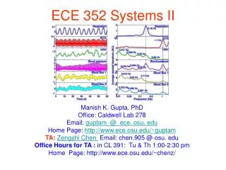
ECE 352 Systems II Manish K. Gupta, PhD Office: Caldwell Lab 278 Email: guptam @ ece. osu. edu Home Page: http://www.ece.osu.edu/~guptam TA:Zengshi Chen Email: chen.905 @ osu. edu Office Hours for TA : in CL 391: Tu & Th 1:00-2:30 pm Home Page: http://www.ece.osu.edu/~chenz/
Acknowledgements • Various graphics used here has been taken from public resources instead of redrawing it. Thanks to those who have created it. • Thanks to Brian L. Evans and Mr. Dogu Arifler • Thanks to Randy Moses and Bradley Clymer
Slides edited from: • Prof. Brian L. Evans and Mr. Dogu Arifler Dept. of Electrical and Computer Engineering The University of Texas at Austin course: EE 313 Linear Systems and Signals Fall 2003
Continuous-Time Domain Analysis • Example: Differential systems • There are n derivatives of y(t) and m derivatives of f(t) • Constants a0, a1, …, an-1 and b0, b1, …, bm • Linear constant-coefficient differential equation • Using short-hand notation,above equation becomes
Continuous-Time Domain Analysis • PolynomialsQ(D) and P(D)where an = 1: • Recall n derivatives of y(t) and m derivatives of f(t) • We will see that this differential system behaves as an (m-n)th-order differentiator of high frequency signals if m > n • Noise occupies both low and high frequencies • We will see that a differentiator amplifies high frequencies. To avoid amplification of noise in high frequencies, we assume that m n
Continuous-Time Domain Analysis • Linearity: for any complex constants c1 and c2,
f(t) T[·] y(t) Continuous-Time Domain Analysis • For a linear system, • The two components are independent of each other • Each component can be computed independently of the other
Zero-input response Response when f(t)=0 Results from internal system conditions only Independent of f(t) For most filtering applications (e.g. your stereo system), we want no zero-input response. Zero-state response Response to non-zero f(t) when system is relaxed A system in zero state cannot generate any response for zero input. Zero state corresponds to initial conditions being zero. Continuous-Time Domain Analysis
Zero-Input Response • Simplest case • Solution: • For arbitrary constant C • Could C be complex? • How is C determined?
Zero-Input Response • General case: • The linear combination of y0(t) and its n successive derivatives are zero. • Assume thaty0(t) = C e l t
Zero-Input Response • Substituting into the differential equation • y0(t) = C el t is a solution provided that Q(l) = 0. • Factor Q(l) to obtain n solutions:Assuming that no two li terms are equal
Zero-Input Response • Could li be complex? If complex, • For conjugate symmetric roots, and conjugate symmetric constants,
Zero-Input Response • For repeated roots, the solution changes. • Simplest case of a root l repeated twice: • With r repeated roots
Characteristic equation Q(D)[y(t)] = 0 The polynomial Q(l) Characteristic of system Independent of the input Q(l) roots l1, l2, …, ln Characteristic roots a.k.a. characteristic values, eigenvalues, natural frequencies Characteristic modes (or natural modes) are the time-domain responses corresponding to the characteristic roots Determine zero-input response Influence zero-state response System Response
L R f(t) C y(t) Envelope RLC Circuit • Component values L = 1 H, R = 4 W, C = 1/40 F Realistic breadboard components? • Loop equations (D2 + 4 D + 40) [y0(t)] = 0 • Characteristic polynomial l2 + 4 l + 40 =(l + 2 - j 6)(l + 2 + j 6) • Initial conditions y(0) = 2 A ý(0) = 16.78 A/s y0(t) = 4 e-2t cos(6t - p/3) A
Linear Time-Invariant System • Any linear time-invariant system (LTI) system, continuous-time or discrete-time, can be uniquely characterized by its • Impulse response: response of system to an impulse • Frequency response: response of system to a complex exponential e j 2 p f for all possible frequencies f • Transfer function: Laplace transform of impulse response • Given one of the three, we can find other two provided that they exist May or may not exist May or may not exist
Impulse response Impulse response of a system is response of the system to an input that is a unit impulse (i.e., a Dirac delta functional in continuous time)
passband Example Frequency Response • System response to complex exponential e jw for all possible frequencies wwherew = 2 p f • Passes low frequencies, a.k.a. lowpass filter |H(w)| H(w) stopband stopband w w -ws -wp wp ws Phase Response Magnitude Response
d[k] k Kronecker Impulse • Let d[k] be a discrete-time impulse function, a.k.a. the Kronecker delta function: • Impulse response h[k]: response of a discrete-time LTI system to a discrete impulse function 1
Zero-State Response • Q(D) y(t) = P(D) f(t) • All initial conditions are 0 in zero-state response • Laplace transform of differential equation, zero-state component
Transfer Function • H(s) is called the transfer function because it describes how input is transferred to the output in a transform domain (s-domain in this case) Y(s) = H(s) F(s) y(t) = L-1{H(s) F(s)} = h(t) * f(t) H(s) = L{h(t)} • The transfer function is the Laplace transform of the impulse response
Transfer Function • Stability conditions for an LTIC system • Asymptotically stable if and only if all the poles of H(s) are in left-hand plane (LHP). The poles may be repeated or non-repeated. • Unstable if and only if either one or both of these conditions hold: (i) at least one pole of H(s) is in right-hand plane (RHP); (ii) repeated poles of H(s) are on the imaginary axis. • Marginally stable if and only if there are no poles of H(s) in RHP, and some non-repeated poles are on the imaginary axis.
Laplace transform Assume input f(t) & output y(t) are causal Ideal delay of T seconds Examples
Ideal integrator with y(0-) = 0 Ideal differentiator with f(0-) = 0 Examples
f(t) f(t) s 1/s F(s) s F(s) F(s) Cascaded Systems • Assume input f(t) and output y(t) are causal • Integrator first,then differentiator • Differentiator first,then integrator • Common transfer functions • A constant (finite impulse response) • A polynomial (finite impulse response) • Ratio of two polynomials (infinite impulse response) f(t) f(t) 1/s s F(s) F(s)/s F(s)
est h(t) y(t) Frequency-Domain Interpretation • y(t) = H(s) e s tfor a particular value of s • Recall definition offrequency response: ej 2p f t h(t) y(t)
Frequency-Domain Interpretation • s is generalized frequency: s = s + j 2 p f • We may convert transfer function into frequency response by if and only if region of convergence of H(s) includes the imaginary axis • What about h(t) = u(t)? We cannot convert this to a frequency response However, this system has a frequency response • What about h(t) = d(t)?
f(t) 1 t Unilateral Laplace Transform • Differentiation in time property f(t) = u(t) What is f ’(0)? f’(t) = d(t).f ’(0) is undefined. By definition of differentiation Right-hand limit, h = h = 0, f ’(0+) = 0 Left-hand limit, h = - h = 0, f ’(0-) does not exist
F(s) W(s) H(s) Y(s) F(s) H1(s) H2(s) Y(s) = F(s) H1(s)H2(s) Y(s) H1(s) = F(s) Y(s) F(s) H1(s) + H2(s) Y(s) H2(s) E(s) F(s) G(s) 1 + G(s)H(s) Y(s) F(s) G(s) Y(s) = - H(s) Block Diagrams
F(s) F(s) H1(s) H2(s) H2(s) H1(s) Y(s) Y(s) Derivations • Cascade W(s) = H1(s)F(s) Y(s) = H2(s)W(s) Y(s) = H1(s)H2(s)F(s) Y(s)/F(s) = H1(s)H2(s) One can switch the order of the cascade of two LTI systems if both LTI systems compute to exact precision • Parallel Combination Y(s) = H1(s)F(s) + H2(s)F(s) Y(s)/F(s) = H1(s) + H2(s)
Feedback System Combining these two equations What happens if H(s) is a constant K? Choice of K controls all poles in the transfer function This will be a common LTI system in Intro. to Automatic Control Class (required for EE majors) Derivations
Many possible definitions Two key issues for practical systems System response to zero input System response to non-zero but finite amplitude (bounded) input For zero-input response If a system remains in a particular state (or condition) indefinitely, then state is an equilibrium state of system System’s output due to nonzero initial conditions should approach 0 as t System’s output generated by initial conditions is made up of characteristic modes Stability
Stability • Three cases for zero-input response • A system is stable if and only if all characteristic modes 0 as t • A system is unstable if and only if at least one of the characteristic modes grows without bound as t • A system is marginally stable if and only if the zero-input response remains bounded (e.g. oscillates between lower and upper bounds) as t
Right-handplane (RHP) Im{l} Stable Unstable Re{l} MarginallyStable Left-handplane (LHP) Characteristic Modes • Distinct characteristic roots l1, l2, …, ln • Where l = s + j win Cartesian form • Units of w are in radians/second
Repeated roots For r repeated roots of value l. For positive k Decaying exponential decays faster thantk increases for any value of k One can see this by using the Taylor Series approximation for elt about t = 0: Characteristic Modes
Stability Conditions • An LTIC system is asymptotically stable if and only if all characteristic roots are in LHP. The roots may be simple (not repeated) or repeated. • An LTIC system is unstable if and only if either one or both of the following conditions exist: (i) at least one root is in the right-hand plane (RHP) (ii) there are repeated roots on the imaginary axis. • An LTIC system is marginally stable if and only if there are no roots in the RHP, and there are no repeated roots on imaginary axis.
f(t) h(t) y(t) Response to Bounded Inputs • Stable system: a bounded input (in amplitude) should give a bounded response (in amplitude) • Linear-time-invariant (LTI) system • Bounded-Input Bounded-Output (BIBO) stable
Impact of Characteristic Modes • Zero-input response consists of the system’s characteristic modes • Stable system characteristic modes decay exponentially and eventually vanish • If input has the form of a characteristic mode, then the system will respond strongly • If input is very different from the characteristic modes, then the response will be weak
Impact of Characteristic Modes • Example: First-order system with characteristic mode el t • Three cases
h(t) 1/RC e-1/RC t t System Time Constant • When an input is applied to a system, a certain amount of time elapses before the system fully responds to that input • Time lag or response time is the system time constant • No single mathematical definition for all cases • Special case: RC filter • Time constant is t = RC • Instant of time at whichh(t) decays to e-1 0.367 of its maximum value
h(t) ĥ(t) h(t0) h(t) t t0 th System Time Constant • General case: • Effective duration is th seconds where area under ĥ(t) • C is an arbitrary constant between 0 and 1 • Choose th to satisfy this inequality • General case appliedto RC time constant:
u(t) h(t) y(t) h(t) u(t) A 1 t t Step Response • y(t) = h(t) * u(t) • Here, tris the rise time of the system • How does the rise time tr relate to the system time constant of the impulse response? • A system generally does not respond to an input instantaneously y(t) A th t tr tr
Filtering • A system cannot effectively respond to periodic signals with periods shorter than th • This is equivalent to a filter that passes frequencies from 0 to 1/th Hz and attenuates frequencies greater than 1/th Hz (lowpass filter) • 1/th is called the cutoff frequency • 1/tr is called the system’s bandwidth (tr = th) • Bandwidth is the width of the band of positive frequencies that are passed “unchanged” from input to output
Transmission of Pulses • Transmission of pulses through a system (e.g. communication channel) increases the pulse duration (a.k.a. spreading or dispersion) • If the impulse response of the system has durationth and pulse had durationtpseconds, then the output will have duration th + tp
Laplace transforms with zero-valued initial conditions Capacitor Inductor Resistor + v(t) – + v(t) + – v(t) – Passive Circuit Elements Transfer Function
First-Order RC Lowpass Filter R + + x(t) C y(t) i(t) Time domain R + + X(s) Y(s) I(s) Laplace domain
Laplace transforms with non-zeroinitial conditions Capacitor Inductor Passive Circuit Elements