Download
1 / 20
220 likes | 250 Views
Explore methods like FFT, Metropolis algorithm, Simplex method, QR algorithm, and more. Understand Fourier Transform, FFT computation complexity, wavelets applications, and more.

E N D
Metropolis algorithm for Monte Carlo • Simplex method for linear programming • Krylov subspace iteration (CG) • Decomposition approach to matrix computation (LU, Singular value) • The Fortran compiler • QR algorithm for eigenvalues • Quick sort • Fast Fourier transform • Integer relation detection • Fast multipole
Convolution, Correlation, and Power Autocorrelation if g = h. Autocorrelation is equal to power spectrum |G(f)|2 in frequency space. Total power:
Sampling Theorem • Let Δ be the spacing in time domain, with hn=h(nΔ), n = …,-2,-1,0,1,2,…, the sampled value of continuous function h(t). Let fc=1/(2Δ) [Nyquist critical frequency]. If H( f ) = 0 for all | f | ≥ fc, then the function h(t) is completely determined by hn.
Aliasing Figure 12.1.1. The continuous function shown in (a) is nonzero only for a finite interval of time T. It follows that its Fourier transform, whose modulus is shown schematically in (b), is not bandwidth limited but has finite amplitude for all frequencies. If the original function is sampled with a sampling interval Δ, as in (a), then the Fourier transform (c) is defined only between plus and minus the Nyquist critical frequency. Power outside that range is folded over or “aliased” into the range. The effect can be eliminated only by low-pass filtering the original function before sampling.
From Continuous to Discrete • Sample time at interval Δ for N points (N even), tk=kΔ, k = 0, 1, 2, …, N-1. • Frequency takes values at fn=n/(NΔ), n=-N/2,-N/2+1, …, 0, 1, 2,…,N/2-1. • Then
Discrete Fourier Transform • Definition • Some properties F is symmetric, FT=F (FT)* F = N I F-1=F*/N (inverse transform is obtained by replacing i with –i, and dividing by N)
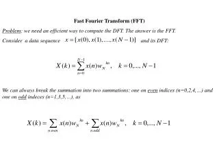
Discrete Fourier Transform – computational complexity • Slow way - O(N2) • Fast way, FFT - O(N log N) • What is the computational complexity of a matrix multiplying a vector, Ax? What if Aij=A(i-j), i.e., a convolution?
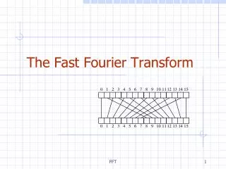
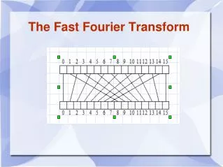
Basic Idea of FFT • Where HN/2,e is the discrete Fourier transform of N/2 points formed from even set of points, and HN/2,o similar but from odd set of points. This calculation is performed recursively.
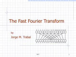
Example for N=8 (A) The order of input data need to be rearranged (according to binary bit-reversed pattern). (B) Values for all k can be evaluated in place. No additional memory is needed.
Example of FFT Swap data according to bit reversal FT of x in place 4= eik 2= eik/2 = eik/4 x0 x0 x0+x4 x0+x4+x2+x6 x0+x4+x2+x6+x1+x5+x3+x7 F2 x1 x4 x0–x4 x0-x4+i(x2-x6) x0-x4+i(x2-x6)+ei/4 (x1-x5+i(x3-x7)) F4 x2 x2 x2+x6 x0+x4-(x2+x6) x0+x4-x2-x6+i(x1+x5-x3-x7) x3 x6 x2–x6 x0-x4-i(x2-x6) x0-x4-i(x2-x6)+ ei3/4(x1-x5-i(x3-x7)) F8 x1+x5 x4 x1 x1+x5+x3+x7 x0+x4+x2+x6-(x1+x5+x3+x7) x5 x5 x1–x5 x1-x5+i(x3-x7) x0-x4+i(x2-x6)-ei/4 (x1-x5+i(x3-x7)) x6 x3 x3+x7 x1+x5-(x3+x7) x0+x4-x2-x6-i(x1+x5-x3-x7) x7 x7 x3–x7 x1-x5-i(x3-x7) x0-x4-i(x2-x6)- ei3/4(x1-x5-i(x3-x7)) Spacing =2 Spacing =4 Spacing =1
Cooley-Tukey bit reversal FFT program FFT runs in O(N log N)
Input Output
Wavelets • Fourier transform is local in frequency domain and nonlocal in time • Wavelet transforms are generalization that is local in both • Discrete wavelet transform is some kind of matrix transform y = Fx, where FTF=I • Wavelets are used in data compression and efficient representation of functions
Daubechies Wavelet Filter F = The coefficients ci are determined by requirements of orthogonality (FTF=I), and certain “vanishing moments”.
Discrete Wavelet Transform F F F Apply F to the upper half of the vector only
Suggested Reading and Software • For a in-depth discussion of FFT algorithms, see C van Loan, “Computational Frameworks for the Fast Fourier Transform” • For state-of-the-art free software, use FFTW at http://www.fftw.org/
Problem set 8 • In the mode-coupling theory of heat transport through materials, one need to solve a set of coupled nonlinear integral-differential equations numerically as follows: • (a) Transform the first equation into frequency domain and solve (algebraically) g in terms of . (b) Describe a procedure to solve the system iteratively using FFT. Where k2 are given, and gk(t) and k(t) are unknown real functions. Dot means time derivative.