Download
1 / 20
200 likes | 417 Views
Wireless & Emerging Networking System Laboratory. Chapter 15. The Fast Fourier Transform. 09 December 2013 Oka Danil Saputra (20136135) IT Convergence Kumoh National Institute of Technology. Fourier Analysis . Represent continuous function by sinusoidal (sine and cosine) functions.

E N D
Wireless & Emerging Networking System Laboratory Chapter 15.The Fast Fourier Transform 09 December 2013 Oka DanilSaputra (20136135) IT Convergence Kumoh National Institute of Technology
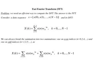
Fourier Analysis • Represent continuous function by sinusoidal (sine and cosine) functions. • Discrete fouriertransform as a sequence function in time domain to another sequence frequency domain .
Fourier Analysis (Cont…) Figure 15.1 (a) A set of 16 data points representing sample of signal strength in the time interval 0 to 2 • Example of the discrete fouriertransform.
Fourier Analysis (Cont…) f3 f4 f2 f1 To calculate the coefficient , for each frequency divide the amplitude by 8 (half of 16, the number of sample point) • The frequency 1 component is 16. • The frequency 2 component is -8. • The frequency 3 component is -16. • The frequency 4 component is 4. Figure 15.1 (b) The discrete fouriertransform yields the amplitude and Frequencies of the constituent sine and cosine functions • The function generating the signal is of the form:
Fourier Analysis (Cont…) Figure 15.1 (c) A plot of the four constituent functions and their sum a continuous function. (d) A plot of the continuous function and the original 16 sample • The generating signal are:
Fourier Analysis (Cont…) Figure 15.2 Discrete fouriertransform for human speech • This plot can be used as inputs to speech recognition system with identify spoken through pattern recognition.
The Discrete Fourier Transform • Given an element vector , the DFT is the matrix-vector product , where is the primitive th root of unity. • Example, compute DFT of the vector (2,3) where the primitive square root of unity is -1. • Compute the DFT of the vector (1,2,4,3) using the primitive fourth root of unity, which is .
The Discrete Fourier Transform (Cont…) • Let’s put the DFT for previous section where we have a vector of 16 complex. • The DFT of this vector is: • To determine the coefficients of the sine and cosine, we examine the nonzero element in the first half. • Thus the combination of sine and cosine functions making up the curve is:
Inverse Discrete Fourier Transform • Given an n element vector x, the inverse DFT is:
Sample Application: Polynomial Multiplication • For example, to multiply the two polynomials. • Yielding: • Convolute the coefficient vectors: • The result:
Sample Application: Polynomial Multiplication (Cont…) Another way to multiply two polynomials of degree n-1 is: To evaluate at the n complex throots of unity. Perform an element-wise multiplication of the polynomials value at these points. Interpolate the results to produce the coefficients of the product polynomial.
Sample Application: Polynomial Multiplication (Cont…) We perform the DFT on the coefficients of p(x). Perform the DFT on the coefficients of q(x).
Sample Application: Polynomial Multiplication (Cont…) 3. We perform an element-wise multiplication. Last step, perform the inverse DFT on the product vector. The vector produced by the inverse DFT contains the coefficients.
The Fast Fourier Transform • The FFT uses a divide-and-conguer strategy to evaluate a polynomial of degree n at the n complex nth roots of unity. • Having Lemma: If is an even positive number, then the squares of the complex th roots of units are identical to the /2 complex (/2)th root of unity.
The Fast Fourier Transform The time complexity of this algorithm is easy to determine. Lets T(n) denote the time needed to perform the FFT on a polynomial of degree n. • The most natural way to express the FFT algorithm is using recursion.
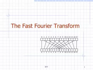
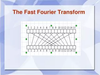
The Fast Fourier Transform (Cont…) Figure 15.4 (a) Recursive implementation of FFT • Figure 15.4 illustrates the derivation of an iterative algorithm from recursive algorithm. • Performing the FFT on input vector (1,2,4,3) produces the result vector (10,-3-,0,-3+).
The Fast Fourier Transform (Cont…) Figure 15.4 (b) Determining which computations are performed for each function invocation • In figure 15.4b we look inside the functions and determine exactly which operations are performed for each invocation. • The expressions of form a+b(c) and a-b(c) correspond the pseudocode statements.
The Fast Fourier Transform (Cont…) Figure 15.4 (c) Tracking the flow of data values • Iterative algorithm: • After an initial permutation step, the algorithm will iterate log n time. • Each iteration corresponds to a horizontal layer in Figure 15.4c. • Within an iteration the algorithm updates value for each of the indices.
The Fast Fourier Transform (Cont…) Iterative algorithm has the same time complexity as the recursive algorithm :