SuperB Positron Production Study with Low Energy e-

1. SuperB Positron Production and Capture with low energy e- Freddy Poirier – LAL R. Chehab, O. Dadoun, P.Lepercq, A. Variola - LAL R. Boni, S.Guiducci, M.Preger, P.Raimondi - LNF For further details please check IPAC 2010: ‘POSITRON PRODUCTION AND CAPTURE BASED ON LOW ENERGY ELECTRONS FOR SUPERB’, THPUB057, F. Poirier et al. and ‘THE INJECTION SYSTEM OF THE INFN-SUPERB FACTORY PROJECT PRELIMINARY DESIGN’, THPEA007, R. Boni et al. and check the talk at the XII SuperB meeting in Annecy: ‘SUPERB POSITRON PRODUCTION AND CAPTURE’ (details of the scenarios) poirier@lal.in2p3.fr

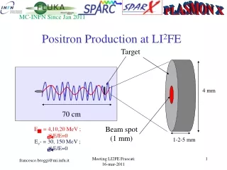
2. SuperB Positron Production Study 10 nC 2.856 GHz ASTRA (Parmela/G4) Geant4 Accelerating Capture Section 2.856 GHz e- (0.6 to 1 GeV) Present study: 600 MeV Tungsten Target ACS W: 1.04 cm thick Freddy poirier 04/06/10

3. Target Yields Studies Target Geant 4 simulation (O. Dadoun – LAL): 1.7 If we increase the energy of the drive beam, the positron yield goes up. For a 600 MeV e- beam, the optimum yield is 1.7 e+/e- with a W-target thickness of 1.04 cm Freddy poirier 04/06/10

4. The AMD • The Adiabatic Matching Device is based on a slowly decreasing magnetic field system which collect the positrons after the target. • AMD has a wide momentum range acceptance (with respect to systems such as Quarter Wave Transformers) • The AMD for the present SuperB Studies is 50 cm long with a longitudinal field Bl starting at Bl(0)=6T decreasing down to Bl(50cm)=0.5T Transverse emittance in AMD is transformed: At exit of AMD: Large Energy Spread Geant 4 Astra Energy (MeV) <E>=~20MeV Erms=~40MeV Px (MeV) Zrms=~2.2cm (tail!) Good agreement (px/pz) Z (m) X (m) Freddy poirier 04/06/10

5. 3.054m Tanks Solenoid ~300MeV Cells The ACS • Accelerating Capture Section (ACS) Goal: Collect and Accelerate positrons up to ~280 MeV. • The ACS is encapsulated in a 0.5 T solenoid and includes several tanks: • Example: • 6 tanks for Full Acceleration at 2.856 GHz – Travelling Wave • 1 tank = 84 cells (+2 couplers), ~3.054m • RF: 2.856 GHz, 2π/3 • 0.9466 cm of aperture (constant radius) P.Lepercq (LAL) has calculated the Travelling Wave Fields in SuperFish and adapted them for ASTRA’s simulation: Field line in a 6 cells TW cavity Freddy poirier 04/06/10

6. The ACS • Several scenarios are under investigation • Accelerating / Deceleration • depending on the type of RF cavities within the ACS • 1st scenario = 2.846 GHz full acceleration • 2nd scenario = 2.846 GHz deceleration + acceleration • 3rd scenario = 1.428 GHz deceleration + acceleration • 4rd scenario = combination of RF types (using 3 GHz TM020 mode for deceleration and 1.428 GHz TM010 for downstream acceleration). These 4 scenarios are under investigation. Scenario 2 and 4 are brought up to 1 GeV Freddy poirier 04/06/10

7. 2.856 GHz: Deceleration scenario • Find the RF phase which gathers a maximum of particles within a bunch • Find the peak gradient which helps this At the exit of the 1st tank: Goal: -Maximise particles in this bunch -Minimise its length -Minimise the other bunches 200o 280o 10MV/m Population Population 280o E (MeV) Z (m) Scenario 2 Note: If the peak gradient in the first cavity used for deceleration is too high, the energy distribution at the exit of the cavity increases  so choice of peak gradient of 10 MV/m

8. A 4th Scenario • 3000 MHz TM020 for Deceleration and 1428 MHz for downstream acceleration (A.Variola) • 1st tank is a 3 GHz tank = 2.93 m • Iris – Aperture larger (Here we constrained the radius opening to 20 mm) • compactified bunch length when deceleration • Shorter beam line for the 3GHz TM020 case (wrt 1428 MHz only) • 2nd up to 4th are 1.428 GHz tank = 6.10 m each • Tank gradient = 25 MV/m (but then modified to 13 MV/m) • Tank phase optimised for maximum acceleration on crest for the considered bunch • Because of the RF (1.428GHz), the wavelength is rather large and the energy dispersion due to acceleration on crest is minimised • 21.84 m from the beginning of the AMD needed here to reach at least 300 MeV Freddy poirier 04/06/10

9. Recap 25MV/m for acceleration • 4 Scenarios under investigation With a positron injection of 10 nC and a yield of 3.9%, we will have 2.43 109 positrons at 300 MeV ±10MeV(scenario 2 – 2.8 GHz) These values are a good indication of how well the scenarios work but need we to bring these to 1 GeV (DR energy)

10. Update on work • Adapt to 13 MV/m for 1.428 GHz RFs • To cope with the difficulty of reaching the peak gradient of 25MV/m at room temperature • ACS (within the 0.5T solenoid) length increases • Slightly lower average energy at end of ACS • Similar results (yield ±10MeV) as before were obtained at ~280 MeV (see IPAC paper) • Extension to 1 GeV • Use of a simple FODO lattice downstream a quadrupole-based matching section Freddy poirier 04/06/10

11. Layout Example Up to ~1050 MeV Acc. Cavity 1.428 GHz, Peak gradient= 13MV/m 3 GHz 10 MV/m Fodo cells 38  ~160 m Solenoid 0.5 T 0.534.1 m Matching section 34.3 ~38 m Freddy poirier 04/06/10

12. At end of the fodo accelerating section 3.0 GHz tank (deceleration), ~1050 MeV At ~160 m, after the target. At exit of last cavity, Particles within a cut radius: Total yield Yield ± 10 MeV Yield (e+/e-) Energy (MeV) 1050 ±10 MeV Radius (m) Z (m) 240 pC 5 mm transverse r-cutYield=~4%

13. Results (Very Preliminary) • For 25 Hz DR filling, we want: • 240 pC per bunch (1.5 109 e+), • Emittance = 3. 10-6 m rad, • Energy acceptance of ±1% (±10MeV) • We have here at present time at 1 GeV (not optimised): some work needed here before optimisation Freddy poirier 04/06/10

14. Further studies at 1 GeV Possible cause: Radial field at the end of the 0.5 T solenoid: Example from 1.428 GHz (scenario 3) Y (m) Dissociation at the end of the solenoid X (m) Cross-plane Coupling !!! Solution: Play on the solenoid field end (use a more adiabatic one) If difficult (because loss of particles): use cross plane correction Radial field

15. Conclusion • A first lattice from target up to ~280 MeV and FODO based lattice up to the DR was built up • Several Energy strategies have been studied as well as several RF scenarios • Some of the Scenarios lead potentially very well to the required yield for the DR • Still a lot of room for optimisation of the lattice • Cross-plane Coupling (Further work needed here. Is CpC a problem? Do we want to correct it?) • Possible global correction based on skew-quads at end of linac • We’ll need a way to connect the end of present linac to the DR such that the particles distribution is given to A. Chancé. • We have not taken into account any “Safety knobs” which would increase the nb of e+ or help to relax requirements such as: • Higher drive e- beam energy • 10 bunches in the DR • Higher DR energy (will reduce the emittance by adiabatic damping) or larger transverse acceptance • AMD length (shorter = 20 cm) and lattice optimisation might give some leverage • Possible DAFNE test under discussion using phase shifter for the first so-called CS tank and adaptation of peak gradient (important asset but can we?) Low energy primary beam can offer a good candidate to provide a sufficient and good quality positron beam. Freddy poirier 04/06/10

16. First order linear design for the main linac, considerations. (H Pascal) Exit from the damping ring : H plane => e= 3.3 10-8 a= 0.47 b = 11.81 V plane =>e = 1.8 10-8 a = 0.52 b =16.14 Use of commercial Qpoles

17. Tested: • Both quadrupoles • 1 / 2 / 3 SLAC cavity period 3,5 / 7 / 10,5 m • Doublet lattice • Best solution found => 2 cavity period FODO, ~ 4.5 T/m • Matching line simple (3 quads)

18. Period, 2 Slac S Band cavities / EMQO-01-200-340 Beam envelope. Final energy 5 GeV

19. Distructive Emittance measurement line 3 gradient method (multiple point) 2 fits : 1parabolic / 2 least squares Phylosophy : 1 scan for both planes But can be modified…. Length ~30 m to have ~ % precision But we started without constraints

20. x y

21. NEXT • Misalignment errors • Full Parmela file • 3 positions method

22. More Slides

23. ACS previous studies (XIth SuperB Meeting) • Full acceleration case simulated with G4+Parmela • But no realistic bunch length out of the AMD • This corresponded to the best we can get for the full acceleration case (without optimisation). - Large impact of the accelerating technology used (mainly due to aperture) - Combined impact of the primary beam + AMD design &We gained flexibility and more realistic bunch length using ASTRA Latest investigations are using ASTRA&

24. ACS energy strategy • 2(extreme) possibleenergy strategy scenario: • Acceleration mode • Straight out of the AMD the particles are accelerated •  we use 25 mV/m • Deceleration mode • The particles are decelerated to form straight a small bunch •  choice of peak gradient for the cavities (free ~10MV/m) Acceleration phase Deceleration phase Exemple with a 1.4 GHz Cavity, 4 MV/m

25. At end of 4th tank – 3000MHz • As an indication: • 333 MeV ± 10 MeV Energy (MeV) 323 343 • 29.4%(1481 positrons) • sz=3.5 mm Note yield for e+ within 331 and 339 MeV = 15.9%

26. At end of 4th tank – 3000MHz • 1st tank is a 3 GHz tank = 2.93 m • 2nd up to 4th are 1.428 GHz tank = 6.10 m each • Tank gradient = 25 MV/m • Tank phase optimised for maximum acceleration on crest for the considered bunch • Because of the RF (1.428GHz), the wavelength is rather large and the energy dispersion due to acceleration on crest is minimised • 21.84 m from the beginning of the AMD needed here to reach at least 300 MeV

27. Simulation Specifics • Tools in use for simulations of the Adiabatic Matching Device (AMD) and the Accelerating Capture Section (ACS): • Parmela (LAL version) • AMD + ACS were simulated initially with Parmela • Though the AMD field inputs for Parmela was rather difficult to modify and to implement (as based on coils) • Some problems, due to lost particles with large angle at entrance of AMD, not resolved. • New Cavity field implementation for Parmela is time consuming. • Geant4(LAL version) • AMD field simulation done (analytical longitudinal and radial field) • No bunch length so far (work in progress) • Astra • AMD field simulation done (analytical) • ACS field with inputs from SuperFish relatively fast to implement • Each code has its drawbacks • Though benchmarks have been done and show relatively good agreement: This work is in progress • Geant4 (AMD) + Parmela (ACS) have been used for the first batch of simulation (continued work) • ASTRA is presently being used to simulate both ACS and AMD. • We gained in flexibility

28. The AMD • Input: • 300 mm bunch out of the target • Yield = 1.7 e+/e- for a 600 MeV e- bunch • Output from the 6T 50 cm long AMD: Large Energy Spread Geant 4 Astra Energy (MeV) <E>=~20MeV Erms=~40MeV Px (MeV) Zrms=~2.2cm (tail!) Good agreement (px/pz) Z (m) X (m)

29. RF in tanks • P.Lepercq (LAL) has calculated the Travelling Wave Fields in SuperFish and adapted them for ASTRA’s simulation: Field line in a 6 cells TW cavity 2π/3 mode Longitudinal field in a single tank (2.8 GHz): Seen by ref. particle 25 MV/m Adaptation and normalisation Adjustment of irises, RF to the required 2π/3 mode, group velocity,.. 1 tank = ~3.054 m Freddy poirier 04/06/10

30. What are the simulated ACS? ACS scenarios: 1 4 2 3 S-Band/L-Band (Dece) S-Band (Acc) S-Band (Dece) L-Band (Dece)

31. 2.856 GHz: Acceleration scenario New results using ASTRA including the zRMS at exit of the AMD of ~2.2 cm End of tank number 6: • End of 1st tank results: Energy (MeV) Population Energy (MeV) Z (m) Energy (MeV) <E>=40MeV Erms=20MeV Zrms=5mm We used here a very stringent cavity phase which limitates the capture Z (m) Z (m) Total yield is 2.8% with an Erms/E of 7% at 300 MeV There is still room for further optimisation in the ACS tanks, we could increase the yield and keep a relatively low Erms.andshort bunch. Scenario 1

32. At end of ACS – 2.856GHz • Full acceleration in downstream tanks (7 in total) is used after deceleration: Zrms=6.4mm Gaussian fit: ~289 ±12 MeV Energy (MeV) Z (m)  Total Yield here: 7.5% Calculated yield for particles within 287±10 MeV:3.9% Scenario 2

33. End of 1st Tank – 1428 MHz • 1 Tank = ~6.10 m • Deceleration mode • 250o • 6 MV/m Scenario 3 Again game is to catch maximum of particles in a small bunch Rather short bunch and low energy distribution Energy (MeV) Energy (MeV) Z (m) Z (m) Gaussian Fit sz = 4.6 mm

34. At end of 4th tank – 1428MHz • Acceleration on crest up to the 4th tank leading to an average energy of roughly 300 MeV ~25m long beam line Energy (MeV) Energy (MeV) sz=8.89 10-03 m se=16.9 (9.09) MeV ( but energy Tails!) sx’=1.69 10-3 rad, sy’=1.74 10-3 rad sx=8.0 10-3 m, sy=8.2 10-3 m Total Yield = ~32.3% Transverse Emittance = 1.35 10-5 rad.m (=sx*sx’), Longitudinal Emittance=0.08 MeV.m (=sz*se)

35. At end of 4th tank – 1428MHz At 1 GeV, we want ± 1% i.e. ±10 MeV of energy dispersion. Having an idea of the yield for ± 10 MeV at 300 MeV gives us an idea of how well our scenario work. • Yield for particles between 300 ± 10 MeV: • 19.6%(994 positrons) • sz=6.4 mm • sx’=1.84 10-3 rad, sy’=1.76 10-3 rad • sx=7.7 10-3 m, sy=8.3 10-3 m Energy (MeV)

36. End of 1st Tank – 3000 MHz Scenario 4 • Length of 1st tank = ~2.93 m • Cell length= 3.331cm • Tank Phase f1= 280o • Tank Gradient G1=10MV/m Gaussian Fit sz = 3.66 10-3 m Energy (MeV) Energy (MeV) Z (m) Z (m)

37. At end of 4th tank – 3000MHz ~21.9 m long beam line • Average Energy = ~333 MeV Energy (MeV) Energy (MeV) sz=3.5 10-03 m se=5.2 (3.2) MeV sx’=1.4 10-3 rad, sy’=1.46 10-3 rad sx=8.1 10-3 m, sy=8.1 10-3 m Z (m) Z (m) Total Yield = ~31.9% Scenario 4

38. Extension to 1 GeV • What are the implications at 1 GeV (DR entrance)? • To get answers: • A simplified lattice was built up with a 0.5 T solenoid extension from 300 MeV up to 1 GeV (total length=~65 m) • Similar model as the lattice up to 300 MeV. • A more complex lattice is under investigation including quadrupoles.

39. Extension to 1 GeV • No optimisation of the simplified lattice (solenoid) • Assumption on the DR requirements: • Implication on the bunch current:

40. Results (Very Preliminary) • For 25 Hz DR filling, we want 240 pC per bunch (1.5 109 e+), Emittance = 3. 10-6 m rad and energy acceptance of ±1% • We have here at present time: • 2.856 GHz (scenario 2) – (some work needed here): • yield of 2.3% (±10 MeV) 1.4 109 • With r-cut = 5 mm  1.5%  ~1.0 109 • 3 GHz + 1.428 GHz (sc. 4): • yield of ~20% (±10 MeV)  12 109 • With r-cut=5 mm  4%  ~2.5 109 Freddy poirier 04/06/10