Download
1 / 33
330 likes | 349 Views
SuperB Positron Production and Capture. Freddy Poirier – LAL R. Chehab, O. Dadoun, P.Lepercq, A. Variola,. poirier@lal.in2p3.fr. SuperB Positron Production Study. e+/e- Target. Primary beam Linac for e - 100s MeV. Pre-injector Linac for e + ~280 MeV. 10 nC. 1 GeV. Damping Ring.

E N D
SuperB Positron Production and Capture Freddy Poirier – LAL R. Chehab, O. Dadoun, P.Lepercq, A. Variola, poirier@lal.in2p3.fr
SuperB Positron Production Study e+/e- Target Primary beam Linac for e- 100s MeV Pre-injector Linac for e+ ~280 MeV 10 nC 1 GeV Damping Ring ~300 MeV 2.856 GHz e- gun AMD Parmela/Astra/G4 Geant4 Accelerating Capture Section 2.856 GHz e- (0.6 to 1 GeV) Present study: 600 MeV Tungsten Target ACS W: 1.04 cm thick
Target Yields Studies Target Geant 4 simulation (O. Dadoun – LAL): 1.7 For a 600 MeV e- beam, the optimum yield is 1.7 e+/e- with a W-target thickness of 1.04 cm Previous studies* were using a yield of 1.58 e+/e- with a target thickness of 1.40 cm * As shown at SuperB 2009 Meeting in Frascati.
The AMD • The Adiabatic Matching Device is based on a slowly decreasing magnetic field system which collect the positrons after the target. • AMD has a wide momentum range acceptance (with respect to systems such as Quarter Wave Transformers) • The AMD for the present SuperB Studies is 50 cm long with a longitudinal field Bl starting at Bl(0)=6T decreasing down to Bl(50cm)=0.5T Transverse emittance in AMD is transformed: 95% Ellipse of actual positrons distribution in AMD Bl(z) (Gauss) Where a = 22. m-1 Z (cm)
The AMD • Input: • 300 mm bunch out of the target • Yield = 1.7 e+/e- for a 600 MeV e- bunch • Output from the 6T 50 cm long AMD: Large Energy Spread Geant 4 Astra Energy (MeV) <E>=~20MeV Erms=~40MeV Px (MeV) Zrms=~2.2cm (tail!) Good agreement (px/pz) Z (m) X (m)
3.054m Tanks Solenoid ~300MeV Cells The ACS • Accelerating Capture Section (ACS) Goal: Collect and Accelerate positrons up to at least 300 MeV. • The ACS is encapsulated in a 0.5 T solenoid and includes several tanks: • Example: • 6 tanks for Full Acceleration at 2.856 GHz – Travelling Wave • 1 tank = 84 cells (+2 couplers), ~3.054m • RF: 2.856 GHz, 2π/3 • 0.9466 cm of aperture (constant radius) • The ACS is here simulated using ASTRA (gain in flexibility) • The positrons are then accelerated up to DR energy requirements (~1 GeV).
RF in tanks • P.Lepercq (LAL) has calculated the Travelling Wave Fields in SuperFish and adapted them for ASTRA’s simulation: Field line in a 6 cells TW cavity 2π/3 mode Longitudinal field in a single tank (2.8 GHz): Seen by ref. particle 25 MV/m Adaptation and normalisation Adjustment of irises, RF to the required 2π/3 mode, group velocity,.. 1 tank = ~3.054 m
The ACS • Capture and Acceleration depends on: • Strategy employed for collecting positrons • A) Full Acceleration • Straight out of the AMD, the particles are accelerated (25MV/m) • B) Deceleration (first cavity) + Acceleration • The positrons are decelerated to form a small bunch (free peak gradient = ~10MV/m) • This gives different scenarios depending on the type of RF cavities within the ACS • 1st scenario = 2.846 GHz full acceleration • 2nd scenario = 2.846 GHz deceleration + acceleration • 3rd scenario = 1.428 GHz deceleration + acceleration • 4rd scenario = (A.Variola’s idea) combination of RF types (using 3 GHz TM020 mode for deceleration and 1.4 GHz TM010 acceleration). This 4 scenarios are under investigation
What are the simulated ACS? ACS scenarios: 1 4 2 3 S-Band/L-Band (Dece) S-Band (Acc) S-Band (Dece) L-Band (Dece)
2.856 GHz: Acceleration scenario New results using ASTRA including the zRMS at exit of the AMD of ~2.2 cm End of tank number 6: • End of 1st tank results: Energy (MeV) Population Energy (MeV) Z (m) Energy (MeV) <E>=40MeV Erms=20MeV Zrms=5mm We used here a very stringent cavity phase which limitates the capture Z (m) Z (m) Total yield is 2.8% with an Erms/E of 7% at 300 MeV There is still room for further optimisation in the ACS tanks, we could increase the yield and keep a relatively low Erms.andshort bunch. Scenario 1
2.856 GHz: Deceleration scenario • Find the RF phase which gathers a maximum of particles within a bunch • Find the peak gradient which helps this At the exit of the 1st tank: Goal: -Maximise particles in this bunch -Minimise its length -Minimise the other bunches 200o 280o 10MV/m Population Population 280o E (MeV) Z (m) Scenario 2
At end of ACS – 2.856GHz • Full acceleration in downstream tanks (7 in total) is used after deceleration: Zrms=6.4mm Gaussian fit: ~289 ±12 MeV Energy (MeV) Z (m) Total Yield here: 7.5% Calculated yield for particles within 287±10 MeV:3.9% Scenario 2
End of 1st Tank – 1428 MHz • 1 Tank = ~6.10 m • Deceleration mode • 250o • 6 MV/m Scenario 3 Again game is to catch maximum of particles in a small bunch Rather short bunch and low energy distribution Energy (MeV) Energy (MeV) Z (m) Z (m) Gaussian Fit sz = 4.6 mm
At end of 4th tank – 1428MHz • Acceleration on crest up to the 4th tank leading to an average energy of roughly 300 MeV ~25m long beam line Energy (MeV) Energy (MeV) sz=8.89 10-03 m se=16.9 (9.09) MeV ( but energy Tails!) sx’=1.69 10-3 rad, sy’=1.74 10-3 rad sx=8.0 10-3 m, sy=8.2 10-3 m Total Yield = ~32.3% Transverse Emittance = 1.35 10-5 rad.m (=sx*sx’), Longitudinal Emittance=0.08 MeV.m (=sz*se)
At end of 4th tank – 1428MHz At 1 GeV, we want ± 1% i.e. ±10 MeV of energy dispersion. Having an idea of the yield for ± 10 MeV at 300 MeV gives us an idea of how well our scenario work. • Yield for particles between 300 ± 10 MeV: • 19.6%(994 positrons) • sz=6.4 mm • sx’=1.84 10-3 rad, sy’=1.76 10-3 rad • sx=7.7 10-3 m, sy=8.3 10-3 m Energy (MeV)
A 4th Scenario • 3000 MHz TM020 for Deceleration and 1428 MHz for acceleration • 1st tank is a 3 GHz tank = 2.93 m • Iris – Aperture larger (Here we constrained the radius opening to 20 mm) • compactified bunch length when deceleration • Shorter beam line for the 3GHz TM020 case (wrt 1428 MHz only) • 2nd up to 4th are 1.428 GHz tank = 6.10 m each • Tank gradient = 25 MV/m • Tank phase optimised for maximum acceleration on crest for the considered bunch • Because of the RF (1.428GHz), the wavelength is rather large and the energy dispersion due to acceleration on crest is minimised • 21.84 m from the beginning of the AMD needed here to reach at least 300 MeV
End of 1st Tank – 3000 MHz Scenario 4 • Length of 1st tank = ~2.93 m • Cell length= 3.331cm • Tank Phase f1= 280o • Tank Gradient G1=10MV/m Gaussian Fit sz = 3.66 10-3 m Energy (MeV) Energy (MeV) Z (m) Z (m)
At end of 4th tank – 3000MHz ~21.9 m long beam line • Average Energy = ~333 MeV Energy (MeV) Energy (MeV) sz=3.5 10-03 m se=5.2 (3.2) MeV sx’=1.4 10-3 rad, sy’=1.46 10-3 rad sx=8.1 10-3 m, sy=8.1 10-3 m Z (m) Z (m) Total Yield = ~31.9% Scenario 4
Recap • 4 Scenarios under investigation With a positron injection of 10 nC and a yield of 3.9%, we will have 2.43 109 positrons at 300 MeV ±10MeV(scenario 2 – 2.8 GHz) These values are a good indication of how well the scenarios work but it’s not enough
Extension to 1 GeV • What are the implications at 1 GeV (DR entrance)? • To get answers: • A simplified lattice was built up with a 0.5 T solenoid extension from 300 MeV up to 1 GeV (total length=~65 m) • Similar model as the lattice up to 300 MeV. • A more complex lattice is under investigation including quadrupoles.
Extension to 1 GeV • No optimisation of the simplified lattice • Assumption on the DR requirements: • Implication on the bunch current:
Conclusion • A first lattice from target up to ~300 MeV and a simplified one to the DR was built up • Several Energy strategies have been studied as well as several RF scenarios • Some of the Scenarios lead to the required yield for the DR • Still a lot of room for optimisation of the lattice • We have not taken into account any “Safety knobs” which would increase the nb of e+ or help to relax requirements such as: • Higher drive e- beam energy • 10 bunches in the DR • Higher DR energy (will reduce the emittance by adiabatic damping) or larger transverse acceptance AMD, lattice optimisation might give some leverage Low energy primary beam can offer a good candidate to provide a sufficient and good quality positron beam.
Pre-Conclusion • Comparisons (preliminary): • Acceleration / Deceleration • Deceleration allows to gain in total Yield • Bunch length shorter, Energy dispersion smaller • 2856 / 1428 MHz • Maximum total Yield for 1428 MHz • Energy dispersion (smaller for 1428MHz) • 1428 / 3000 (TM020) MHz • 1st tank: • Total Yield higher for 1428 MHz • Same particle density (to be shown properly) • Shorter beamline for 3000 MHz
ACS previous studies (XIth SuperB Meeting) • Full acceleration case simulated with G4+Parmela • But no realistic bunch length out of the AMD • This corresponded to the best we can get for the full acceleration case (without optimisation). - Large impact of the accelerating technology used (mainly due to aperture) - Combined impact of the primary beam + AMD design &We gained flexibility and more realistic bunch length using ASTRA Latest investigations are using ASTRA&
ACS’s RF cavities • The Accelerating Capture Section (ACS) is encapsulated in a 0.5 T solenoid and includes 7 tanks (6 for full acceleration scenario) • 1 tank = 85 cells, ~3.054m • RF: 2.856 GHz, 2π/3 • 0.9466 cm of aperture (constant radius) • Pierre Lepercq (LAL) calculated the field for the Travelling waves using SuperFish Exemple including the field lines with the 6 cells travelling wave for Parmela Simulation:
ACS energy strategy • 2(extreme) possibleenergy strategy scenario: • Acceleration mode • Straight out of the AMD the particles are accelerated • we use 25 mV/m • Deceleration mode • The particles are decelerated to form straight a small bunch • choice of peak gradient for the cavities (free ~10MV/m) Acceleration phase Deceleration phase Exemple with a 1.4 GHz Cavity, 4 MV/m
Comparison – end of 1st tank • short tank length (3GHz) • shorter bunch length (3GHz) • same density of particles for a given short z size • More particles (1.4GHz) • smaller energy dispersion (1.4GHz not surprising)
At end of 4th tank – 3000MHz • As an indication: • 333 MeV ± 10 MeV Energy (MeV) 323 343 • 29.4%(1481 positrons) • sz=3.5 mm Note yield for e+ within 331 and 339 MeV = 15.9%
At end of 4th tank – 3000MHz • 1st tank is a 3 GHz tank = 2.93 m • 2nd up to 4th are 1.428 GHz tank = 6.10 m each • Tank gradient = 25 MV/m • Tank phase optimised for maximum acceleration on crest for the considered bunch • Because of the RF (1.428GHz), the wavelength is rather large and the energy dispersion due to acceleration on crest is minimised • 21.84 m from the beginning of the AMD needed here to reach at least 300 MeV
AMD (6 T – 50 cm) exit Population Energy (MeV) Energy distribution at the exit from the AMD, using Geant4 simulation
Deceleration Approach • Idea from SLAC in the late 70’s (SLAC-pub-2393) • Arranging the phase and amplitude of the fields so that the distribution in longitudinal phase space of the incoming positrons lay along one of the orbits in longitudinal phase space:
Simulation Specifics • Tools in use for simulations of the Adiabatic Matching Device (AMD) and the Accelerating Capture Section (ACS): • Parmela (LAL version) • AMD + ACS were simulated initially with Parmela • Though the AMD field inputs for Parmela was rather difficult to modify and to implement (as based on coils) • Some problems, due to lost particles with large angle at entrance of AMD, not resolved. • New Cavity field implementation for Parmela is time consuming. • Geant4(LAL version) • AMD field simulation done (analytical longitudinal and radial field) • No bunch length so far (work in progress) • Astra • AMD field simulation done (analytical) • ACS field with inputs from SuperFish relatively fast to implement • Each code has its drawbacks • Though benchmarks have been done and show relatively good agreement: This work is in progress • Geant4 (AMD) + Parmela (ACS) have been used for the first batch of simulation (continued work) • ASTRA is presently being used to simulate both ACS and AMD. • We gained in flexibility