Download
1 / 15
150 likes | 279 Views
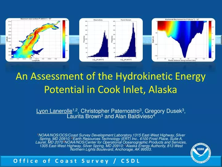
An Assessment of the Hydrokinetic Energy Potential in Cook Inlet, Alaska. Lyon Lanerolle 1,2 , Christopher Paternostro 3 , Gregory Dusek 3 , Laurita Brown 3 and Alan Baldivieso 4

E N D
An Assessment of the Hydrokinetic Energy Potential in Cook Inlet, Alaska Lyon Lanerolle1,2, Christopher Paternostro3, Gregory Dusek3, Laurita Brown3 and Alan Baldivieso4 1NOAA/NOS/OCS/Coast Survey Development Laboratory,1315 East-West Highway, Silver Spring, MD 20910; 2Earth Resources Technology (ERT) Inc., 6100 Frost Place, Suite A, Laurel, MD 2070; 3NOAA/NOS/Center for Operational Oceanographic Products and Services, 1305 East-West Highway, Silver Spring, MD 20910; 4Alaska Energy Authority, 813 West Northern Lights Boulevard, Anchorage, AK 99503.
Introduction and Motivation • Alaska Energy Authority (AEA) interested in optimal locations for siting hydrokinetic energy projects in Cook Inlet, AK • AEA-NOAA/National Ocean Service (NOS) partnership established • NOAA/NOS/CO-OPS performed field study in Summer 2012 with ADCPs • NOAA/NOS/CSDL performed model simulations to complement field study • Two model studies : Phase 1 - constant density, tides only (Jan-Feb 2008) Phase 2 - full synoptic hindcast (Jan-Aug 2012) • Phase 2 modeled currents evaluated against field observations • Numerical model output fields seamless - well suited for producing maps, etc. • Final assessment from modeling study will provide AEA with guidance on turbine placement, etc.
Field Study Areas and Modeling Domains • Field study had 9 current meters (magenta circles – south to north) • Model has one parent domain (blue) • Also two high resolution nests • Kachemak Bay nest (red) • Upper Cook Inlet nest (green) • Model nesting technology previously established at NOAA/NOS/OCS/CDSL • Model nesting – one way
Numerical Model Set-up • Use Rutgers University’s Regional Ocean Modeling System (ROMS) • Phase 1 run for 36 days beginning 01/01/2008 with constant density & tidal forcing only • Phase 2 run from 01/01/2012 – 08/31/2012 with variable density and multiple model forcings(spun-up from rest as before) • Initialization - T and S (WOA-2001 climatology) • River - discharge and T (USGS gauges) • Open boundary - sub-tidal water level (GRTOFS) • Open boundary - T and S (WOA-2001 climatology) • Surface boundary - ROMS bulk flux (NAM06 products) • ~6 months allowed for flow-field to develop before model-obs evaluation
Currents Evaluation and Validation - 1 • Currents analyzed at mid-water depth (to avoid surface/bottom effects) • Analyze major-axis component (along Principal Current Direction) • Plot Spring cycle to maximize contrast • Currents errors mainly in amplitudes • Errors more pronounced in upper Cook Inlet – model under-predicts amplitudes • Errors also from model &obs having different tidal constituent compositions Blue - obs, Red - parent grid, Green - KB nest, Magenta - up CI nest
Currents Evaluation and Validation - 2 Currents Amplitude Errors • Use autocorrelation-based amplitude-phase error splitting technique • Amplitude error accuracy ± 0.001 m (1 mm) • Parent grid – slight error dependence on station location • KB nest gives slightly better results than parent grid • Upper CI nest gives slightly worse results than parent grid • Errors ~7% - 21% relative to Spring cycle amplitude (from obs.) & no pattern • Modeled currents are sufficiently accurate
Currents Evaluation and Validation - 3 Currents Phase Errors • Phase errors from amplitude-phase error splitting technique • Phase error accuracy ± 1.0 minutes • Parent grid – errors less than ~20 min., lagging in KB and leading in upper CI • KB nest - similar errors to parent grid and also lagging • Upper CI nest - smaller errors than parent grid and also leading • Amplitude and phase errors relatively large at station 3 – nesting boundary effects
Maximum Power Density on Parent Grid Near surface Mid-water Near-bottom • Power Density, P=0.5*ρ*|U|3 where |U|=(u2 + v2)1/2 as w << u, v; [P] = W/m2 • Plot P in Log10 scale for clarity and contrast • Highest P near surface and lowest near bottom but similar distributions (≈ x 1/30) • Geographically, highest P : along axis of Cook Inlet, North Foreland, strait between West Foreland and East Foreland (and some isolated locations in upper CI) • Maximum P ~ 30 kW/m2 • Similar to Phase I results – ~90% of currents signal is purely tidal!
Maximum Power Density on Nested Grids Kachemak Bay Upper Cook Inlet • Comparison for near-surface fields • Parentand Nested grids show similar Power Densities • Differences mainly for Kachemak Bay • Little power within Kachemak Bay • Upper Cook Inlet is energetic • Similar to fields from Phase 1 Parent Parent Nest Nest
Vertical Distribution of Power Density Nest Phase 1 Parent Nest Nest Phase 1 Parent Nest • Transects are time snapshots • Parent and nested domains give similar results • Kachemak Bay less energetic and upper Cook Inlet more energetic • Phase 2 KB transects more stratified and show met forcing effects • Upper CI transects similar to each other – dominated by strong currents
Power Extraction Times (Near-Surface) Parent Parent Parent Grid Parent Grid Phase 1 KB Nest up CI Nest • PE time = available time (hrs.) to extract at least 1 kW/m2over 31-days of July, 2012 • Can set threshold(1 kW/m2) to any value • Can choose any depth for analysis • Phase 2 allows consistently longer extraction times over Phase 1 – Strait between E and W Foreland, N. Foreland, Point Possession, channels above Fire Island and within Knik Arm (“hot spots”) • PE times between parent and nested domains similar but also some differences (KB nest) • Highest PE time areas allow 500-600 hours of extraction – i.e. ~70%-80% of the time • Perhaps most useful metric for deciding placement of turbines
Assessing Power Density Accuracy - 1 • P = 0.5 ρ |U|3→ΔP/P = 3 Δ|U|/|U| • Relative error in P is x 3 relative error in |U| (speed) • 1% error in |U| →3% error in P &3.3% error in |U| →10% error in P! • Generating 3.3% accuracy currents throughout a model domain with a Hydrodynamic modelis unrealistic! • With mid-water depth, major-axis currents errors in |U| ≈7%-21% → errors in P ≈21%-63% - which is significant • Error analysis assumes observed currents are error-free
Assessing Power Density Accuracy - 2 • Examine power densities from observed and modeledmid-water depth currents • Currents time-series covered July 16 – August 16, 2012 • Plot power density histograms on Log10 scale for contrast • Calculate & compare mean power densities - modeled mean vs. observed mean • Mean/STD for obs. & model are 1693/2365& 1439/1752 (kW/m2) • Spread (due to tides) too large → Means not reliable • Same for all 9 current stations Mean
Assessing Power Density Accuracy - 3 • Calculate extraction times with obs. and modeled mid-water currents (Jul-Aug, 2012) • Very meaningful/useful metric • 1 kW/m2 power density threshold used • Little energy in Kachemak Bay (station 1) • Parent grid compares better with obs. than nests • Reasonable model – obs. agreement except stations 7 and 8 – could be bathymetry, sediment • Modeled times shorter than obs. times • For obs. in KB PD threshold crossed <30% of the time but in upper CI its >50% • Less power available at mid-water depths than near-surface region
Conclusions • Second, fully synoptic hindcast(Phase 2) conducted to complement constant density, tides only initial simulation (Phase 1) - for hydrokinetic energy assessment of Cook Inlet • Modeled currents evaluated against observations & found to be reasonably accurate • Parent grid power densities & extraction times in agreement with those from nested grids • Nested grids did not generate more accurate results – one-way nesting may not be enough & may need 2-way nesting • Phase 2 and Phase 1 power densities in agreement - ~90% of current signal is purely tidal. Some differences seen in power density vertical stratification • Phase 2 and Phase 1 power extraction times also in agreement. Phase 2 allowed relatively longer extraction times • Little energy in Kachemak Bay. Localized energy “hot spots” in upper Cook Inlet where power density of 1 kW/m2 or greater available for 70%-80% of the time • As power density is proportional to speed cubed- need extremely accurate currents to get accurate power density estimates • Due to tidal action, power density histograms can not be used to compute reliable means • At mid-water depths got reasonable model – observations agreement for extraction times. Less energy available than near-surface regions • Energy/Power analysis techniques developed here generally applicable