Download

1 / 42
440 likes | 658 Views
A Hybrid Artificial Neural Network Model with Linear & Nonlinear Components. Yolcu Ufuk, ( varyansx@hotmail.com ) Department of Statistics, Giresun University, Giresun 28000, Turkey, Egrioglu Erol ( erole@omu.edu.tr ) Department of Statistics, Ondokuz Mayis University, Samsun 55139, Turkey

E N D
A Hybrid Artificial Neural Network Model with Linear&Nonlinear Components Yolcu Ufuk, (varyansx@hotmail.com) Department of Statistics, Giresun University, Giresun 28000, Turkey, Egrioglu Erol (erole@omu.edu.tr) Department of Statistics, Ondokuz Mayis University, Samsun 55139, Turkey Aladag Cagdas H. (chaladag@gmail.com) Department of Statistics, Hacettepe University, Ankara 06800, Turkey
CONTENT • Introduction • The Proposed Method (L&NL-ANN Model) • Application of L&NL-ANN Model 3.1. Data Set 1 3.2. Data Set 2 • Conclusions
Introduction • In the literature, while linear models such as autoregressive integrated moving average (ARIMA; [2]) have being used for linear time series, nonlinear models such as artificial neural networks (ANN), bilinear, and threshold autoregressive (TAR; [15]) have being preferred for nonlinear time series. • It is a well-known fact that real life time series can generally contain both linear and non-linear components. • It is almost impossible that a time series is pure linear or pure nonlinear.
For some time series, linear models can produce satisfactory results when linear part of the time series is superior to nonlinear part. • In a similar way, when nonlinear part of the time series is superior to linear part, nonlinear models can give satisfactory results. • However, in both case, one of these parts is not taken into consideration. • Thus, it can lead to deceptive results. • To deal with this problem, various hybrid approaches have been suggested in theliterature.
Tseng et al. (2002) proposed a hybrid forecasting model, which combines the seasonal ARIMA (SARIMA) and ANN [16]. • Zhang (2003) improved a hybrid model based on ARIMA and ANN [20]. • Pai and Lin (2005) combined ARIMA and support vector machines (SVM) [12]. • Chen and Wang (2007) combined SARIMA and SVM [4]. • Aladag et al. (2009) combined ARIMA and Elman neural networks [1].
Lee and Tong (2011) combined ARIMA and genetic algorithms [9]. • Besides, Ince and Traffalis (2006) proposed a hybrid model which incorporates parametric techniques such as ARIMA, vector autoregressive (VAR) and co-integration techniques, and nonparametric techniques such as support vector regression (SVR) and ANN [6]. • Wang et al. (2006) introduced some hybrid approaches which are called threshold ANN, cluster based ANN, and periodic ANN [18].
BuHamra et al. (2003) and Jain and Kumar (2007) suggested hybrid approaches in which the inputs of ANN are determined by Box-Jenkins procedure ([3]; [7]). • In addition to these studies, hybrid approaches combine SARIMA and ANN also proposed to analyze fuzzy time series by Egrioglu et al. (2009) and Uslu et al. (2010) ([5]; [17]).
These hybrid approaches generally consist of two phases. • After linear component of time series is modeled with a linear model in the first phase, nonlinear component is modeled by utilizing a nonlinear model in the next phase. • In two-phase methods, it is assumed that time series has only linear structure in the first phase and it is assumed that time series has only nonlinear structure in the second phase. • Therefore, this causes model specification error.
In this study, a new ANN model composed of both linear and nonlinear structures is proposed to deal with this problem and to increase forecasting accuracy. • Therefore, this method has the ability to model both linear and nonlinear parts in time series at the same time. • In the proposed model, Multiplicative and Mc Culloch-Pitts neuron structures are used for nonlinear and linear parts, respectively. • In addition, the modified particle swarm optimization (MPSO) method is used to train the proposed neural network model.
To show the applicability of the proposed method, it is applied to two real life time series in the implementation. • For the aim of comparison, the obtained results are compared to those calculated from other approaches available in the literature. • As a result of the implementation, it is seen that the proposed method has the best forecasting accuracy.
2. The Proposed Method Hybridmodels include advantages of both linear and nonlinear models have also been proposed in the literature. In hybrid approaches, it is assumed that the time series is composed of sum of linear and nonlinear parts and can be defined by where yt, Lt, and Nt represent the time series, the linear part and the nonlinear part of the time series, respectively.
In the literature, Zhang (2003), Pai and Lin (2005), Chen and Wang (2007), Aladag et al. (2009) and Lee and Tong (2011) employed two-phase hybrid approaches. • After the linear part of time series is modeled in the first phase, by assuming that residuals obtained in the first phase contain the nonlinear part, these residuals are analyzed with nonlinear models in the second phase. • Employing a linear model in the first phase means that nonlinear relations are not taken into consideration. • This situation causes model specification error.
To overcome this problem, one-phase method which can simultaneously analyze both linear and nonlinear structures is needed when time series given in (1) are analyzed. • Therefore, a novel linear & nonlinear artificial neural network (L&NL-ANN) model is proposed in this study. • The broad structure of the proposed model is illustrated in Fig. 2.1.
In Fig. 2.1, ∑ and ∏ represent neuron models Mc Culloch and Pitts, and multiplicative neuron models, respectively. The functions f1 and f2 are given in (2) and (3), respectively. • As seen in Fig. 2.1, L&NL-ANN model includes two components linear and nonlinear.
W1 is a vector that includes the weights between the inputs of the linear component and neurons in the hidden layer corresponding to the linear part of the model. • Similarly, the vector W2 contains the weights between the inputs of the nonlinear component and neurons in the hidden layer corresponding to the nonlinear part of the model. • Each component has m inputs so both W1 and W2 are mx1. The vector W3, which is 2x1, consists of two weights which are used to combine outputs calculated from linear and nonlinear components.
Thus, calculation of the output of L&NL-ANN model is given in three stages. Stage 1. The output value of the neuron in the hidden layer corresponding to the linear component (o1) is calculated. Firstly, the activation value net1 for the neuron is obtained by using the formula given as follows: where w1j (j=1,2,…,m) are elements of W1, and b1 is bias weight for the linear part. The activation function used in this neuron is f1 given in (2) so the output value o1 is calculated by
Stage 2. The output value of the neuron in the hidden layer corresponding to the nonlinear component (o2) is calculated. Before calculating o2, the activation value net2 for the neuron is computed by using the formula given in (6). where w2j, and b2j (j=1,2,…,m) are elements of W2, and bias weight values for the nonlinear part. The activation function used in this neuron is f2 given in (3) so the output value o2 is calculated by
Stage 3. The output value of the model is calculated. First of all, the activation value net3 for the neuron in the output layer is obtained by using the formula given in (8). In (8), b3 is bias weight. Then, the output value is computed as follows: As seen from (9), the output value is obtained from the weighted sum of linear and nonlinear autoregressive models. Unlike the model given in (1), L&NL-ANN model can be expressed as in (10).
It should be noted in here that in the model given in (1), weights of linear and nonlinear components are equal. However, in L&NL-ANN model, these weights are determined during the optimization process of ANN due to the structure of the data. In the proposed approach, L&NL-ANN model, which is also defined in this study, is trained using MPSO method. In the MPSO, positions of a particle are weights of L&NL-ANN model. Hence, a particle has 3m + 4 positions. Structure of a particle is illustrated in Fig. 2.2.
Mean square error (MSE), which is a well-known forecasting performance criterion, is used as evaluation function. MSE can be calculated using the formula given in (11). where n represents the number of learning sample. The algorithm for calculation of the output value of the proposed L&NL-ANN model is presented below.
Algorithm: The algorithm for calculation of the output value of the proposed L&NL-ANN model. Step 1. The parameters of MPSO are determined. In the first step, the parameters which direct the MPSO algorithm are determined. These parameters are pn,vm,c1i, c1f, c2i, c2f, w1, and w2 that were given in the [10] and [13]. Step 2. Initial values of positions and velocities are determined. The initial positions and velocities of each particle in a swarm are randomly generated from uniform distribution (0,1) and (-vm,vm), respectively.
Step 3. Evaluation function values are computed. Evaluation function values for each particle are calculated. MSE given in (11) is used as evaluation function. Step 4. Pbestk (k = 1,2, …, pn) and Gbest are determined due to evaluation function values calculated in the previous step. Pbestk is a vector stores the positions corresponding to the kth particle’s best individual performance, and Gbest is the best particle, which has the best evaluation function value, found so far.
Step 5.The parameters are updated. The updated values of cognitive coefficient c1, social coefficient c2, and inertia parameter w are calculated like in [10] and [13]. Step6. New values of positions and velocities are calculated. New values of positions and velocities for each particle are computed like in [10] and [13]. If maximum iteration number is reached, the algorithm goes to Step 3; otherwise, it goes to Step 7. Step 7.The optimal solution is determined. The elements of Gbest are taken as the optimal weight values of the L&NL-ANN.
3. Application of L&NL-ANN Model In order to evaluate the performance of the proposed approach based on the L&NL-ANN model, which also defined in this study, and the MPSO algorithm, the proposed approach is applied to two real time series in the implementation. In all computations, MATLABversion 7.12.0 (R2011a) computer package was used.
3.1 Data Set 1 The first time series is the amount of carbon dioxide measured monthly in Ankara capitol of Turkey (ANSO) between March 1995 and April 2006. It has both trend and seasonal components and its period is 12. The first 124 observations are used for training and the last 10 observations are used for test set.
In addition to the proposed approach, • Seasonal Autoregressive Integrated Moving Average (SARIMA), • Winters Multiplicative Exponential Smoothing (WMES), • Feed Forward Neural Networks (FFANN) methods and the fuzzy time series forecasting methods proposed by Song [14], Egrioglu [5] and Uslu [17] are used to analyze ANSO data. For the test set, the forecasts and root mean square error (RMSE) values produced by all methods are summarized in Table 3.1.
Table 3.1 The obtained results for ANSO data The results of the methods SARIMA, WMES, Song [14], Egrioglu et al. [5] and Uslu et al. [17] were taken from Uslu et al.s’ study.
When FFANN is used, the numbers of neurons in both the hidden and input layers are changed from 1 to 12 and one output neuron is employed. The best architecture among them is found as the architecture contains 12 neurons in the input layer and one neuron in the hidden layer. Thus, the inputs of the best FFANN model are the lagged variables Xt-1, Xt-2, …, Xt-12. Inputs of L&NL-ANN model are taken as Xt-1, Xt-2, …, Xt-12 like in the FFANN model.
And, in the training process of L&NL-ANN model, the parameters of the modified particle swarm optimization are determined as follows:(c1i, c1f) = (2, 3), (c2i, c2f) = (2, 3), (w1, w2) = (1, 2), pn = 30, and maxt = 1000. According to Table 3.1, the proposed approach has the best forecasting accuracy for ANSO data in terms of RMSE. To examine the results visually, the graph of the real observations and the forecasts produced by the proposed approach for test set is given in Fig. 3.1
Fig. 3.1 The graph of observations and forecasts for test data As clearly seen from this graph, the proposed approach produces very accurate forecasts for ANSO data.
3.1 Data Set 2 L&NL-ANN model is also applied to Canadian lynx data consisting of the set of annual numbers of lynx trappings in the Mackenzie River District of North-West Canada for the period from 1821 to 1934. This data has also been extensively analyzed in the time series literature. We use the logarithm (to the base 10) of the data in the analysis.
In addition to the proposed approach, logarithm of Canada lynx data is examined by using the methods proposed by Zhang [20], Katijani et al. [8], Pai and Lin[12], Aladag et al. [1]. When the proposed method is used, the order of the L&NL-ANN model is m=3. MSE values obtained from the methods are presented in Table 3.2. Table 3.2 The obtained MSE values for Test Data of Logarithmic Canadian Lynx Data.
As seen from Table 3.2, the best forecasts are obtained when L&NL-ANN model is used. The graph of the real observations and the forecasts obtained from the proposed approach for test set is given in Fig. 3.2.
Fig. 3.2 The graph of observations and forecasts for test data of data set 2 It is clearly seen from the graph that the forecasts produced by the proposed approach are very accurate.
5. Conclusions It is a well-known fact that real life time series can contain both linear and nonlinear structures. In the literature, various hybrid approaches, which are generally two-phase methods, have been proposed to deal with such time series. After linear component of time series is modeled with a linear model in the first phase, nonlinear component is modeled by utilizing a nonlinear model in the next phase.
In two-phase methods, it is assumed that time series has only linear structure in the first phase and it is assumed that time series has only nonlinear structure in the second phase. Therefore, this causes model specification error. To overcome this problem and to reach high forecasting accuracy level, a new ANN model which can simultaneously analyze both linear and nonlinear structures is introduced in this study.
This model can be considered as one-phase hybrid approach. In the other hybrid approaches available in the literature, weights of linear and nonlinear components are equal. Unlike the other hybrid approaches suggested in the literature, in the proposed neural network model, weights of linear and nonlinear components are determined during the optimization process of ANN due to the structure of the data.
In the proposed model, Multiplicative and Mc Culloch-Pitts neuron structures are used for nonlinear and linear parts, respectively. To show forecasting performance of the proposed method, it is applied to two real life time series in the implementation. As a result of the implementation, it is clearly observed that the proposed method produced the best forecasts for these two real time series.
References 1. Aladag, C.H., Egrioglu, E., Kadilar, C.: Forecasting nonlinear time series with a hybrid methodology, Applied Mathematic Letters, 22, 1467-1470 (2009). 2. Box, G.E.P., Jenkins, G.M.: Time Series Analysis: Forecasting and Control Holdan-Day, San Francisco, CA, (1976). 3. BuHamra, S., Smaoui, N., Gabr, M.: The Box-Jenkins analysis and neural networks: prediction and time series modeling, Applied Mathematical Modeling, 27, 805-815 (2003). 4. Chen, K.Y., Wang, C.H.: A Hybrid SARIMA and support vector machines in forecasting the production values of the machinery industry in Taiwan, Expert Systems with Applications, 32(1), 254-264 (2007). 5. Egrioglu, E., Aladag, C.H., Yolcu, U., Basaran, M.A., Uslu, V.R.: A new hybrid approach based on SARIMA and partial high order bivariate fuzzy time series forecasting model, Expert Systems with Applications, 36, 7424-7434 (2009). 6. Ince, H., Traffalis, T.B.: A hybrid model for exchange rate prediction, Decisions Support Systems, 42, 1054-1062 (2006). 7. Jain, A. Kumar, A.M.; Hybrid neural network models for hydrological time series forecasting, Applied Soft Computing, 7, 585-592 (2007). 8. Katijani, Y., Hipel, W.K. Mcleod, A.I.: Forecasting nonlinear time series with feed forward neural networks: A case study of Canadian Lynx Data, Journal of Forecasting, 24 105-117 (2005). 9. Lee, Y-S., Tong, L-I.: Forecasting time series using a methodology based on autoregressive integrated moving average and genetic programming, Knowledge-Based Systems, 24, 66-72 (2011).
10. Ma, Y., Jiang, C., Hou, Z., Wang, C.: The formulation of the optimal strategies for the electricity producers based on the particle swarm optimization algorithm, IEEE Trans Power System, 21(4):1663–71 (2006). 11. Mc Culloch, W.S., Pitts, W.: A logical calculus of the ideas immanent in nervous activity. Bulletin of Mathematical Biophysics, 5, 115–133 (1943). 12. Pai, P.F., Lin, C.S.: A Hybrid ARIMA and support vector machines model in stock price forecasting, Omega, 33(6), 497-505 (2005). 13. Shi, Y, Eberhart, R.C.: Empirical study of particle swarm optimization. Proc IEEE Int Congr Evol Comput, 3:101–6 (1999). 14. Song, Q.: Seasonal forecasting in fuzzy time series. Fuzzy Sets and Systems, 107, 235–236 (1999). 15. Tong, H.: Non-linear time series: A Dynamical system approach, New York, Oxford University Press (1990). 16. Tseng, F.M., Yu, H.C., Tzeng, G.H.: Combining neural network model with seasonal time series ARIMA model, Technological Forecasting&Social Change, 69, 71-87 (2002). 17. Uslu, V.R., Aladag, C.H., Yolcu, U., Egrioglu, E.: A new hybrid approach for forecasting a seasonal fuzzy time series, International Symposium Computing Science and Engineering Proceeding Book, 1152-1158 (2010). 18. Wang, W., VanGelder, P.H.A.J.M., Vrijling, J.K., Ma, J.: Forecasting daily stream flow using hybrid ANN models, Journal of Hydrology, 324, 383-399 (2006). 19. Yadav, R.N., Kalra, P.K., John, J.: Time series prediction with single multiplicative neuron model, Applied Soft Computing, 7, 1157-1163 (2007). 20. Zhang, G.: Time series forecasting using a hybrid ARIMA and neural network model, Neurocomputing, 50, 159-175 (2003).