Cost Theory Break-Even versus Contribution Analysis

Cost Theory Break-Even versus Contribution Analysis Lecture 5 Econ 340H Managerial Economics Web Appendix 5A Christopher Michael Trent University Department of Economics

Topics • Break-even analysis and operating leverage • Risk assessment

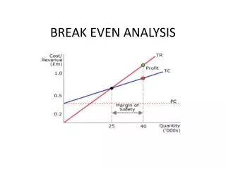
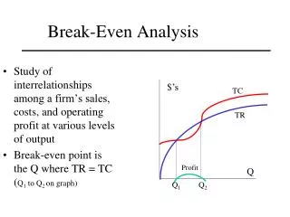
Break-Even Analysis • We can have multiple B/E (break-even) points with non-linear costs & revenues. • If linear total cost and total revenue: TR = P•Q TC = F + V•Q • where V is Average Variable Cost • F is Fixed Cost • Q is Output • Cost-Volume-Profit analysis Total Cost Total Revenue Q B/E B/E

The Break-Even Quantity: Q B/E • At break-even: TR = TC So, P•Q = F + V•Q • Q B/E = F / ( P - V) = F/CM where contribution margin is: CM = ( P - V) TR TC PROBLEM: As a garage contractor, find Q B/E if: P = $9,000 per garage V = $7,000 per garage & F = $40,000 per year Q B/E

Amount of sales revenues that breaks even P•Q B/E = P•[F/(P-V)] = F / [ 1 - V/P ] Answer: QB/E = 40,000/(2,000)= 40/2 = 20 garages at the break-even point. Break-Even Sales Volume Ex: At Q = 20, B/E Sales Volume is $9,000•20 = $180,000 Sales Volume Variable Cost Ratio

Target Profit Output • Quantity needed to attain a target profit • If is the target profit, Q target = [ F + ] / (P-V) Suppose want to attain $50,000 profit, then, Q target = ($40,000 + $50,000)/$2,000 = $90,000/$2,000 = 45 garages

Degree of Operating Leverageor Operating Profit Elasticity • DOL = E sensitivity of operating profit (EBIT) to changes in output • Operating  = TR-TC = (P-V)•Q - F • Hence, DOL = (Q)•(Q/) = (P-V)•(Q/) = (P-V)•Q / [(P-V)•Q - F] A measure of the importance of Fixed Cost or Business Risk to fluctuations in output

DOL as Operating Profit Elasticity DOL = (P - V) Q / [ (P - V) Q - F ] • We can use empirical estimation methods to find operating leverage • Elasticities can be estimated with double log functional forms • Use a time series of data on operating profit and output • Ln EBIT = a + b• Ln Q, where b is the DOL • then a 1% increase in output increases EBIT by b% • b tends to be greater than or equal to 1

DOL = (9,000-7,000) • 45 . [(9,000-7,000)•45 – 40,000] = 90,000 / 50,000 = 1.8 A 1% INCREASE in Q  1.8% INCREASE in operating profit. At the break-even point, DOL is INFINITE. A small change in Q increases EBIT by an astronomically large percentage rate Suppose the Contractor Builds 45 Garages, What is the D.O.L?

Regression Output • Dependent Variable: Ln EBIT uses 20 quarterly observations N = 20 The log-linear regression equation is Ln EBIT = - .75 + 1.23 Ln Q Predictor Coeff Stdev t-ratio p Constant -.7521 0.04805 -15.650 0.001 Ln Q 1.2341 0.1345 9.175 0.001 s = 0.0876 R-square= 98.2% R-sq(adj) = 98.0% The DOL for this firm is 1.23. So, a 1% increase in output leads to a 1.23% increase in operating profit

Operating Profit and the Business Cycle peak EBIT = operating profit Output TIME recession Trough 2. EBIT tends to collapse late in recessions 1. EBIT is more volatile than output over cycle

Break-Even Analysis and Risk Assessment • One approach to risk, is the probability of losing money. • Let QB/E be the break-even quantity, and Q is the expected quantity produced. • z is the number of standard deviations away from the mean • z = (QB/E - Q )/ • 68% of the time within 1 standard deviation • 95% of the time within 2 standard deviations • 99% of the time within 3 standard deviations Continued…

Break-Even Analysis and Risk Assessment (concluded) Problem:If the break-even quantity is 5,000, and the expected number produced is 6,000, what is the chance of losing money if the standard deviation is 500? Answer: z = (5,000 – 6,000) / 500 = -2. There is less than 2.5% chance of losing money. Using table 13B.1, the exact answer is 0.0228 or 2.28% chance of losing money.

Cost Theory Break-Even versus Contribution Analysis