Download
1 / 27
400 likes | 1.16k Views
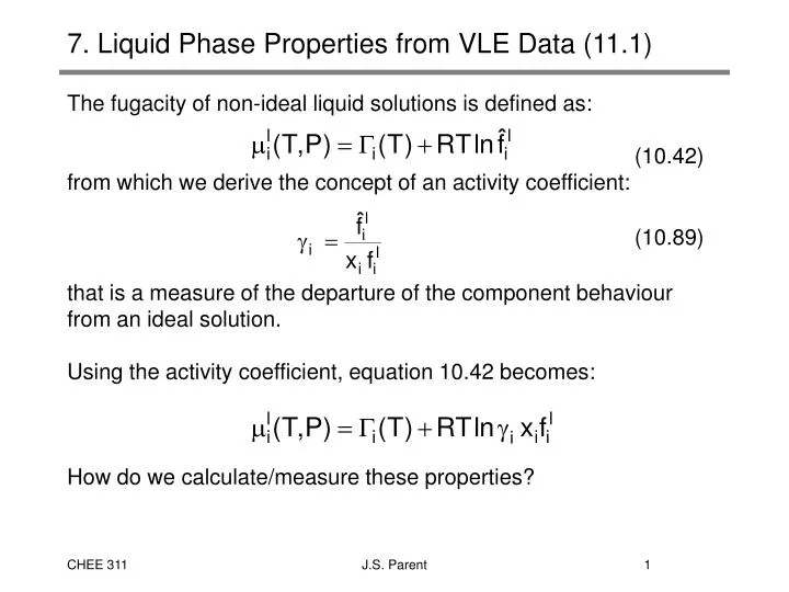
7. Liquid Phase Properties from VLE Data (11.1). The fugacity of non-ideal liquid solutions is defined as: (10.42) from which we derive the concept of an activity coefficient: (10.89)

E N D
7. Liquid Phase Properties from VLE Data (11.1) • The fugacity of non-ideal liquid solutions is defined as: • (10.42) • from which we derive the concept of an activity coefficient: • (10.89) • that is a measure of the departure of the component behaviour from an ideal solution. • Using the activity coefficient, equation 10.42 becomes: • How do we calculate/measure these properties? J.S. Parent
Liquid Phase Properties from VLE Data • Suppose we conduct VLE experiments on our system of interest. • At a given temperature, we vary the system pressure by changing the cell volume. • Wait until equilibrium is established (usually hours) • Measure the compositions of the liquid and vapour J.S. Parent
Liquid Solution Fugacity from VLE Data • Our understanding of molecular dynamics does not permit us to predict non-ideal solution fugacity, fil . We must measure them by experiment, often by studies of vapour-liquid equilibria. • Suppose we need liquid solution fugacity data for a binary mixture of A+B at P,T. At equilibrium, • The vapour mixture fugacity for component i is given by, • (10.47) • If we conduct VLE experiments at low pressure, but at the required temperature, we can use the perfect gas mixture model, • by assuming that iv = 1. J.S. Parent
Liquid Solution Fugacity from Low P VLE Data • Since our experimental measurements are taken at equilibrium, • according to the perfect gas mixture model • What we need is VLE data at various pressures (all relatively low) J.S. Parent
Activity Coefficients from Low P VLE Data • With a knowledge of the liquid solution fugacity, we can derive activity coefficients. Actual fugacity • Ideal solution fugacity • Our low pressure vapour fugacity simplifies fil to: • and if P is close to Pisat: • leaving us with J.S. Parent
Activity Coefficients from Low P VLE Data • Our low pressure VLE data can now be processed to yield experimental activity coefficient data: J.S. Parent
Activity Coefficients from Low P VLE Data J.S. Parent
7. Correlation of Liquid Phase Data • The complexity of molecular interactions in non-ideal systems makes prediction of liquid phase properties very difficult. • Experimentation on the system of interest at the conditions (P,T,composition) of interest is needed. • Previously, we discussed the use of low-pressure VLE data for the calculation of liquid phase activity coefficients. • As practicing engineers, you will rarely have the time to conduct your own experiments. • You must rely on correlations of data developed by other researchers. • These correlations are empirical models (with limited fundamental basis) that reduce experimental data to a mathematical equation. • In CHEE 311, we examine BOTH the development of empirical models (thermodynamicists) and their applications (engineering practice). J.S. Parent
Correlation of Liquid Phase Data • Recall our development of activity coefficients on the basis of the partial excess Gibbs energy : • where the partial molar Gibbs energy of the non-ideal model is provided by equation 10.42: • and the ideal solution chemical potential is: • Leaving us with the partial excess Gibbs energy: • (10.90) J.S. Parent
Correlation of Liquid Phase Data • The partial excess Gibbs energy is defined by: • In terms of the activity coefficient, • (10.94) • Therefore, if as practicing engineers we have GE as a function of P,T, xn (usually in the form of a model equation) we can derive i. • Conversely, if thermodynamicists measure i, they can calculate GE using the summability relationship for partial properties. • (10.97) • With this information, they can generate model equations that practicing engineers apply routinely. J.S. Parent
Correlation of Liquid Phase Data • We can now process this our MEK/toluene data one step further to give the excess Gibbs energy, • GE/RT = x1ln1 + x2ln2 J.S. Parent
Correlation of Liquid Phase Data • Note that GE/(RTx1x2) is reasonably represented by a linear function of x1 for this system. This is the foundation for correlating experimental activity coefficient data J.S. Parent
Correlation of Liquid Phase Data • The chloroform/1,4-dioxane system exhibits a negative deviation from Raoult’s Law. • This low pressure VLE data can be processed in the same manner as the MEK/toluene system to yield both activity coefficients and the excess Gibbs energy of the overall system. J.S. Parent
Correlation of Liquid Phase Data • Note that in this example, the activity coefficients are less than one, and the excess Gibbs energy is negative. • In spite of the obvious difference from the MEK/toluene system behaviour, the plot of GE/x1x2RT is well approximated by a line. J.S. Parent
8.4 Models for the Excess Gibbs Energy • Models that represent the excess Gibbs energy have several purposes: • they reduce experimental data down to a few parameters • they facilitate computerized calculation of liquid phase properties by providing equations from tabulated data • In some cases, we can use binary data (A-B, A-C, B-C) to calculate the properties of multi-component mixtures (A,B,C) • A series of GE equations is derived from the Redlich/Kister expansion: • Equations of this form “fit” excess Gibbs energy data quite well. However, they are empirical and cannot be generalized for multi-component (3+) mixtures or temperature. J.S. Parent
Symmetric Equation for Binary Mixtures • The simplest Redlich/Kister expansion results from C=D=…=0 • To calculate activity coefficients, we express GE in terms of moles: n1 and n2. • And through differentiation, • we find: J.S. Parent
7. Excess Gibbs Energy Models • Practicing engineers find most of the liquid-phase information needed for equilibrium calculations in the form of excess Gibbs Energy models. These models: • reduce vast quantities of experimental data into a few empirical parameters, • provide information an equation format that can be used in thermodynamic simulation packages (Provision) • “Simple” empirical models • Symmetric, Margule’s, vanLaar • No fundamental basis but easy to use • Parameters apply to a given temperature, and the models usually cannot be extended beyond binary systems. • Local composition models • Wilsons, NRTL, Uniquac • Some fundamental basis • Parameters are temperature dependent, and multi-component behaviour can be predicted from binary data. J.S. Parent
Excess Gibbs Energy Models • Our objectives are to learn how to fit Excess Gibbs Energy models to experimental data, and to learn how to use these models to calculate activity coefficients. J.S. Parent
Margule’s Equations • While the simplest Redlich/Kister-type expansion is the Symmetric Equation, a more accurate model is the Margule’s expression: • (11.7a) • Note that as x1 goes to zero, • and from L’hopital’s rule we know: • therefore, • and similarly J.S. Parent
Margule’s Equations • If you have Margule’s parameters, the activity coefficients are easily derived from the excess Gibbs energy expression: • (11.7a) • to yield: • (11.8ab) • These empirical equations are widely used to describe binary solutions. A knowledge of A12 and A21 at the given T is all we require to calculate activity coefficients for a given solution composition. J.S. Parent
van Laar Equations • Another two-parameter excess Gibbs energy model is developed from an expansion of (RTx1x2)/GE instead of GE/RTx1x2. The end results are: • (11.13) • for the excess Gibbs energy and: • (11.14) • (11.15) • for the activity coefficients. • Note that: as x10, ln1 A’12 • and as x2 0, ln2 A’21 J.S. Parent
Local Composition Models • Unfortunately, the previous approach cannot be extended to systems of 3 or more components. For these cases, local composition models are used to represent multi-component systems. • Wilson’s Theory • Non-Random-Two-Liquid Theory (NRTL) • Universal Quasichemical Theory (Uniquac) • While more complex, these models have two advantages: • the model parameters are temperature dependent • the activity coefficients of species in multi-component liquids can be calculated from binary data. • A,B,C A,B A,C B,C • tertiary mixture binary binary binary J.S. Parent
Wilson’s Equations for Binary Solution Activity • A versatile and reasonably accurate model of excess Gibbs Energy was developed by Wilson in 1964. For a binary system, GE is provided by: • (11.16) • where • (11.24) • Vi is the molar volume at T of the pure component i. • aij is determined from experimental data. • The notation varies greatly between publications. This includes, • a12 = (12 - 11), a12 = (21 - 22) that you will encounter in Holmes, M.J. and M.V. Winkle (1970) Ind. Eng. Chem.62, 21-21. J.S. Parent
Wilson’s Equations for Binary Solution Activity • Activity coefficients are derived from the excess Gibbs energy using the definition of a partial molar property: • When applied to equation 11.16, we obtain: • (11.17) • (11.18) J.S. Parent
Wilson’s Equations for Multi-Component Mixtures • The strength of Wilson’s approach resides in its ability to describe multi-component (3+) mixtures using binary data. • Experimental data of the mixture of interest (ie. acetone, ethanol, benzene) is not required • We only need data (or parameters) for acetone-ethanol, acetone-benzene and ethanol-benzene mixtures • The excess Gibbs energy is written: • (11.22) • and the activity coefficients become: • (11.23) • where ij = 1 for i=j. Summations are over all species. J.S. Parent
Wilson’s Equations for 3-Component Mixtures • For three component systems, activity coefficients can be calculated from the following relationship: • Model coefficients are defined as (ij = 1 for i=j): J.S. Parent
Comparison of Liquid Solution Models Activity coefficients of 2-methyl-2-butene + n-methylpyrollidone. Comparison of experimental values with those obtained from several equations whose parameters are found from the infinite-dilution activity coefficients. (1) Experimental data. (2) Margules equation. (3) van Laar equation. (4) Scatchard-Hamer equation. (5) Wilson equation. J.S. Parent