Download
1 / 34
340 likes | 353 Views
This article explores the space-time analogy in geometric optics and its application in pulse/beam shapes, paraxial approximation, Fourier transforms, Gaussian beams, and the use of q parameters and matrices. It also discusses diffraction, dispersion, chirp, and the meaning of k"d in the image plane. Additionally, it covers the application of space-time analogy in fs communication and the use of time lenses and dispersion in fs lasers.

E N D
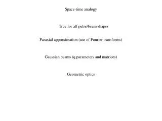
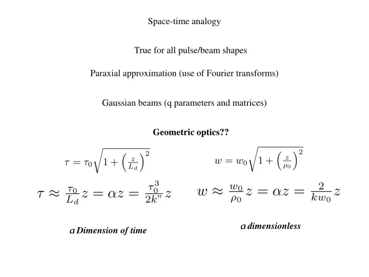
Space-time analogy True for all pulse/beam shapes Paraxial approximation (use of Fourier transforms) Gaussian beams (q parameters and matrices) Geometric optics?? a dimensionless a Dimension of time
SPACE TIME Fourier transform in time Fourier transform in space
Space-time analogy Geometric optics d1 d2 SPACE e(-r/M) e(r) DIFFRACTION DIFFRACTION By matrices:
Space-time analogy Geometric optics d1 d2 TIME e(--t/M) e(t) DISPERSION DISPERSION By matrices: y length in time T = chirp imposed on the pulse
Space-time analogy Gaussian optics d1 d2 SPACE e(-r/M) e(r) DIFFRACTION DIFFRACTION By matrices:
Space-time analogy Gaussian optics d1 d2 TIME e(--t/M) e(t) DISPERSION DISPERSION By matrices: = chirp imposed on the pulse Find the image plane:
WHAT IS THE MEANING k”d? Lf Fiber L Prism Lg b Gratings d Fabry-Perot at resonance
TIME MICROSCOPE d1 d2 e(-r/M) e(r) DIFFRACTION DIFFRACTION e(t) d2 DISPERSION d1 e1(t) TIME LENS DISPERSION
CHIRPED PUMP ep(t) = eeiat 2 TIME LENS e1(t) DISPERSED INPUT TIME LENS OUTPUT w1 wp w1 + e1(t)eiat 2 wp
e e ( - ) ( ) r/M r e ( ) t e e e ( ( ( - - - ) ) ) t/M t/M t/M x x d d d d 1 1 2 2 image image object object e e e e ( ( - - ) ) ( ( ) ) r/M r/M r r (a) (a) diffraction diffraction diffraction diffraction e e ( ( ) ) t t TIME TIME LENS LENS (b) (b) dispersion dispersion dispersion dispersion
Space-time analogy – application to fs communication FEMTOSECOND COMMUNICATION: Commercial fs lasers – a pulse duration of 50 fs. (20 THz) One can easily “squeeze” a 12 bit word in 1 ps
Propagationof time- multiplexed signals EMITTER RECEIVER 1 ns 1 ns 1 ns 1 ns Time stretcher Time compressor time time, ps 0 4 3 2 1
Time “telescope” (reducing) Time “microscope” (expanding)
y’’ L n2
L d g Gaussian mirror (localized gain) In terms of modes, this cavity is equivalent to
Chirp evolution using ABCD matrix in time Cavity in time Cavity in space Dispersion Kerr f = R/2
Damping effect Ti:Saph laser with wavelength at 795nm, beam waist of 211μm, cavity length d = 89cm and equivalent radius of curvature R = 92.5cm. The damping coefficient is = 0.01. Ti:Saph laser with wavelength at 770nm, pulse width about 100fs and pulse energy fixed around 27.5nJ. The Ti:Saph crystal is 3mm long with a Kerr coefficient of 10.5×10⁻¹⁶ cm2/W. The dispersion of the cavity is -800fs2. The damping coefficient is = 0.01.
Oscillating solution and damping If p1 starts with some departure from equilibrium: = Damping in a real laser results from the balance of gain and losses. Mathematically introduce a phenomenological damping coefficient ε Ti:Saph laser with wavelength at 770nm, pulse width about 100fs and pulse energy fixed around 27.5nJ. The Ti:Saph crystal is 3mm long with a Kerr coefficient of 10.5×10⁻¹⁶ cm2/W. The dispersion of the cavity is -800fs2. The damping coefficient ε = 0.01. (does not affect the oscillation period)
L d Saturable gain off-resonance: g (localized gain) No more Gaussian No more damping required
y’’ Gaussian approximation no longer valid L Paraxial still valid F n2 L d g A (localized gain)
y’’ L F n2 L d g A (localized gain)
SPACE TIME Fourier transform in time Fourier transform in space