Constraining Inflation Trajectories with the CMB & Large Scale Structure

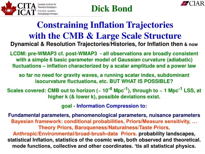
1. Constraining Inflation Trajectories with the CMB & Large Scale Structure Dynamical & Resolution Trajectories/Histories, for Inflation then & now LCDM: pre-WMAP3 cf. post-WMAP3 - all observations are broadly consistent with a simple 6 basic parameter model of Gaussian curvature (adiabatic) fluctuations – inflation characterized by a scalar amplitude and a power law so far no need for gravity waves, a running scalar index, subdominant isocurvature fluctuations, etc. BUT WHAT IS POSSIBLE? Scales covered: CMB out to horizon (~ 10-4 Mpc-1), through to ~ 1 Mpc-1 LSS, at higher k (& lower k), possible deviations exist. goal -Information Compression to: Fundamental parameters, phenomenological parameters, nuisance parametersBayesian framework: conditional probabilities, Priors/Measure sensitivity, … Theory Priors, Baroqueness/Naturalness/Taste Priors, Anthropic/Environmental/broad-brush-data Priors. probability landscapes, statistical Inflation, statistics of the cosmic web, both observed and theoretical. mode functions, collective and other coordinates. ‘tis all statistical physics. Dick Bond

2. CMBology Inflation Histories (CMBall+LSS) subdominant phenomena (isocurvature, BSI) Secondary Anisotropies (tSZ, kSZ, reion) Foregrounds CBI, Planck Polarization of the CMB, Gravity Waves (CBI, Boom, Planck, Spider) Non-Gaussianity (Boom, CBI, WMAP) Dark Energy Histories (& CFHTLS-SN+WL) Probing the linear & nonlinear cosmic web

3. CMB/LSS Phenomenology • Dalal • Dore • Kesden • MacTavish • Pfrommer • Shirokov • CITA/CIAR there • Mivelle-Deschenes (IAS) • Pogosyan (U of Alberta) • Prunet (IAP) • Myers (NRAO) • Holder (McGill) • Hoekstra (UVictoria) • van Waerbeke (UBC) • CITA/CIAR here • Bond • Contaldi • Lewis • Sievers • Pen • McDonald • Majumdar • Nolta • Iliev • Kofman • Vaudrevange • Huang • El Zant • UofT here • Netterfield • MacTavish • Carlberg • Yee • & Exptal/Analysis/Phenomenology Teams here & there • Boomerang03 • Cosmic Background Imager • Acbar • WMAP (Nolta, Dore) • CFHTLS – WeakLens • CFHTLS - Supernovae • RCS2 (RCS1; Virmos-Descart) Parameter datasets:CMBall_pol SDSS P(k), 2dF P(k) Weak lens (Virmos/RCS1; CFHTLS, RCS2) Lya forest (SDSS) SN1a “gold” (157, 9 z>1), CFHT futures: ACT SZ/opt, Spider. Planck, 21(1+z)cm

4. I N F L A T I O N the nonlinear COSMIC WEB • Secondary Anisotropies • Non-Linear Evolution • Weak Lensing • Thermal and Kinetic SZ effect • Etc. • Primary Anisotropies • Tightly coupled Photon-Baryon fluid oscillations • viscously damped • Linear regime of perturbations • Gravitational redshifting Decoupling LSS reionization 19 Mpc 13.7-10-50Gyrs 10Gyrs 13.7Gyrs today

5. Standard Parameters of Cosmic Structure Formation Period of inflationary expansion, quantum noise  metricperturbations Scalar Amplitude Density of Baryonic Matter Spectral index of primordial scalar (compressional) perturbations Spectral index of primordial tensor (Gravity Waves) perturbations Density of non-interacting Dark Matter Cosmological Constant Optical Depth to Last Scattering Surface When did stars reionize the universe? Tensor Amplitude What is the Background curvature of the universe? • Inflation  predicts nearly scale invariant scalar perturbations and background of gravitational waves • Passive/adiabatic/coherent/gaussian perturbations • Nice linear regime • Boltzman equation + Einstein equations to describe the LSS closed flat open

6. New Parameters of Cosmic Structure Formation tensor (GW) spectrum use order M Chebyshev expansion in ln k, M-1 parameters amplitude(1), tilt(2), running(3),... scalar spectrum use order N Chebyshev expansion in ln k, N-1 parameters amplitude(1), tilt(2), running(3), … (or N-1 nodal point k-localized values) Dual Chebyshev expansion in ln k: Standard 6 is Cheb=2 Standard 7 is Cheb=2,Cheb=1 Run is Cheb=3 Run & tensor is Cheb=3, Cheb=1 Low order N,M power law but high order Chebyshev is Fourier-like

7. New Parameters of Cosmic Structure Formation Hubble parameter at inflation at a pivot pt =1+q, the deceleration parameter history order N Chebyshev expansion, N-1 parameters (e.g. nodal point values) Fluctuations are from stochastic kicks ~ H/2p superposed on the downward drift at Dlnk=1. Potential trajectory from HJ (SB 90,91):

8. tensor (gravity wave) power to curvature power, r, a direct measure of e= (q+1), q=deceleration parameter during inflation q (ln Ha) may be highly complex (scanning inflation trajectories) many inflaton potentials give the same curvature power spectrum, but the degeneracy is broken if gravity waves are measured (q+1) =~ 0 is possible - low energy scale inflation – upper limit only Very very difficult to get at this with direct gravity wave detectors – even in our dreams Response of the CMB photons to the gravitational wave background leads to a unique signature within the CMB at large angular scales of these GW and at a detectable level. Detecting these B-modes is the new “holy grail” of CMB science. Inflation prior: on e only 0 to 1 restriction, < 0 supercritical possible GW/scalar curvature: current from CMB+LSS: r < 0.6 or < 0.25(.28)95%;good shot at0.0295% CL with BB polarization (+- .02 PL2.5+Spider), .01 target BUT foregrounds/systematics?? But r-spectrum. But low energy inflation

9. CBI pol to Apr’05 Quiet2 Bicep CBI2 to Apr’07 (1000 HEMTs) Chile QUaD Quiet1 Acbar to ~Jan’06 SCUBA2 APEX Spider (12000 bolometers) (~400 bolometers) Chile SZA JCMT, Hawaii (2312 bolometer LDB) (Interferometer) California ACT Clover (3000 bolometers) Chile Boom03 2017 CMBpol 2003 2005 2007 2004 2006 2008 SPT WMAP ongoing to 2009 ALMA (1000 bolometers) South Pole (Interferometer) Chile DASI Polarbear Planck CAPMAP (300 bolometers) California AMI (84 bolometers) HEMTs L2 GBT

10. WMAP3 thermodynamic CMB temperature fluctuations Like a 2D Fourier transform, wavenumber Q ~ L+½ (~ kperpc)

11. TT, EE, BB, TE, TB, EB Angular Power Spectra

12. WMAP3 sees 3rd pk, B03 sees 4th

13. CBI combined TT sees 5th pk (Dec05,~Mar06)

14. CBI combined TT data (Dec05,~Mar06)

15. high L frontier: CBI/BIMA/ACBAR excess&σ8primarycf.σ8SZ on the excess as SZ; also SZA (consistent with s8=1), APEX, ACT, SPT (Acbar) CBI excess as SZ σ8Bond et al. =0.99±0.10, Komatsu & Seljak =0.90±0.11, Subha etal06 low-z cut =0.85±0.10 s8=.71 +- .05, .77 +- .04 noSZ, .72+-.05 (GW), .80 +.03 (GW+LSS) s8=.80 +- .04 run (-0.05 +- .025) Does not include errors from non-Gaussianity of clusters

16. σ8 Tension of WMAP3 CBI excess as SZ σ8Bond et al. =0.99±0.10, Komatsu & Seljak =0.90±0.11, Subha etal06 low-z cut =0.85±0.10 Subha etal.06 is designed to be consistent with the latest Chandra M-T relation (Vikhlinin etal.06). but latest XMM M-T (Arnaud et al.05) is higher than Chandra. cf. weak lensing CFHTLS survey’05: 0.86 +- .05 + Virmos-Descart & non-G errors s8 = 0.80 +- .04 if Wm = 0.3 +- .05 SZ treatment does not include errors from non-Gaussianity of clusters, uncertainty in faint source counts

17. CBI2 “bigdish” upgrade June2006 + GBT for sources • Caltech, NRAO, Oxford, CITA, Imperial by about Feb07 s8primary s8SZ SZE Secondary CMB Primary ~ s87 on the excess as SZ; SZA, APEX, ACT, SPT (Acbar) will also nail it

18. E and B polarization mode patterns Blue = + Red = - E=“local” Q in 2D Fourier space basis B=“local” U in 2D Fourier space basis Tensor (GW) + lensed scalar Scalar + Tensor (GW) WMAP3 V band CBIpol’05 E cf. B in uv (Fourier) plane

19. Polarization EE:2.5 yrs of CBI, Boom03,DASI,WMAP3 (CBI04, DASI04, CAPmap04 @ COSMO04) & DASI02 EE & WMAP3’06 Phenomenological parameter analysis Lsound@dec vs As CBI+B03+DASI EE,TE cf. CMB TT [Montroy et al. astro-ph/0507514] [Sievers et al. astro-ph/0509203] [Piacentini et al. astro-ph/0507507] [Readhead et al. astro-ph/0409569] [MacTavish et al. astro-ph/0507503]

20. Does TT Predict EE (& TE)? (YES, incl wmap3 TT) Inflation OK: EE (& TE) excellent agreement with prediction from TT pattern shift parameter0.998 +- 0.003 WMAP3+CBIt+DASI+B03+ TT/TE/EE pattern shift parameter1.002 +- 0.0043 WMAP1+CBI+DASI+B03 TT/TE/EE Evolution: Jan00 11% Jan02 1.2% Jan03 0.9% Mar03 0.4% EE: 0.973 +- 0.033, phase check of CBI EE cf. TT pk/dip locales & amp EE+TE 0.997 +- 0.018CBI+B03+DASI (amp=0.93+-0.09)

21. forecast Planck2.5 100&143 Spider10d 95&150 Synchrotron pol’n < .004 ?? Dust pol’n < 0.1 ?? Template removals from multi-frequency data

22. forecast Planck2.5 100&143 Spider10d 95&150 GW/scalar curvature: current from CMB+LSS: r < 0.6 or < 0.2595% CL;good shot at0.0295% CL with BB polarization (+- .02 PL2.5+Spider Target .01) BUT Galactic foregrounds & systematics??

23. SPIDER Tensor Signal • Simulation of large scale polarization signal No Tensor Tensor http://www.astro.caltech.edu/~lgg/spider_front.htm

24. Inflation Then Trajectories & Primordial Power Spectrum Constraints Constraining Inflaton Acceleration TrajectoriesBond, Contaldi, Kofman & Vaudrevange 06 Ensemble of Kahler Moduli/Axion Inflations Bond, Kofman, Prokushkin & Vaudrevange 06

25. Constraining Inflaton Acceleration TrajectoriesBond, Contaldi, Kofman & Vaudrevange 06 “path integral” over probability landscape of theory and data, with mode-function expansions of the paths truncated by an imposed smoothness (Chebyshev-filter) criterion [data cannot constrain high ln k frequencies] P(trajectory|data, th) ~ P(lnHp,ek|data, th) ~ P(data| lnHp,ek ) P(lnHp,ek | th) / P(data|th) Likelihood theory prior / evidence Data: CMBall (WMAP3,B03,CBI, ACBAR, DASI,VSA,MAXIMA) + LSS (2dF, SDSS, s8[lens]) Theory prior uniform inlnHp,ek (equal a-prior probability hypothesis) Nodal points cf. Chebyshev coefficients (linear combinations) monotonic inek The theory prior matters alot We have tried many theory priors

26. Old view: Theory prior = delta function of THE correct one and only theory New view: Theory prior = probability distribution on an energy landscape whose features are at best only glimpsed, huge number of potential minima, inflation the late stage flow in the low energy structure toward these minima. Critical role of collective geometrical coordinates (moduli fields) and of branes and antibranes (D3,D7). Ensemble of Kahler Moduli/Axion Inflations Bond, Kofman, Prokushkin & Vaudrevange 06 A Theory prior in a class of inflation theories thatseem to work Low energy landscape dominated by the last few (complex) moduli fields T1 T2 T3 U1 U2 U3 associated with the settling down of the compactification of extra dims(complex) Kahler modulus associated with a 4-cycle volume in 6 dimensional Calabi Yau compactifications in Type IIB string theory. Real & imaginary parts are both important. Builds on the influential KKLT, KKLMT moduli-stabilization ideas for stringy inflation and the Conlon and Quevada focus on 4-cycles. As motivated and protectedas any inflation model. Inflation: there are so many possibilities: Theory prior ~ probability of trajectories given potential parameters of the collective coordinatesX probability of the potential parameters. X probability of initial collective field conditions

27. TheParameters of Cosmic Structure Formation

28. String Theory Landscape& Inflation++ Phenomenology for CMB+LSS running index as simplest breaking, radically broken scale invariance, 2+-field inflation, isocurvatures, Cosmic strings/defects, compactification & topology, & other baroque add-ons. subdominant String/Mtheory-motivated, extra dimensions, brane-ology, reflowering of inflaton/isocon models (includes curvaton), modified kinetic energies, k-essence, Dirac-Born-Infeld [sqrt(1-momentum**2), “DBI in the Sky” Silverstein etal 2004], etc. Potential of the Hybrid D3/D7 Inflation Model f|| fperp KKLT, KKLMMT any acceleration trajectory will do?? q (ln Ha) H(ln a,…) V(phi,…) Measure?? anti-baroque prior 14 std inflation parameters + many many more e.g. “blind” search for patterns in the primordial power spectrum

29. Kahler/axion moduli Inflation Conton & Quevedo hep-th/0509012 Ensemble of Kahler Moduli/Axion Inflations Bond, Kofman, Prokushkin & Vaudrevange 06: T=t+iq imaginary part (axion q) of the modulus is impt. q gives a rich range of possible potentials & inflation trajectories given the potential

30. Sample trajectories in a Kahler modulus potential t vs q T=t+iq “quantum eternal inflation” regime stochastic kick > classical drift Sample Kahler modulus potential

31. another sample Kahler modulus potential with different parameters (varying 2 of 7) & different ensemble of trajectories

32. Bond, Contaldi, Kofman, Vaudrevange 06 N=-ln(a/ae), k ~ Ha , e = (1+q), e = dlnH/dN, Ps ~ H2 /e, Pt ~ H2 V(f) ~ MPl2 H2 (1-e/3) , f|| = inflaton collective coordinate, d f|| ~ +- sqrt(e)dN

33. Beyond P(k): Inflationary trajectories HJ + expand about uniform acceleration, 1+q, V and power spectra are derived

34. Trajectories cf. WMAP1+B03+CBI+DASI+VSA+Acbar+Maxima + SDSS + 2dF Chebyshev 7 & 10 H(N) and RG Flow 7 10

35. r(ln a)/16 = -nt/2 /(1-nt/2) + small = (1+q) + small

36. Chebyshev nodal modes(order 3, 5, 15) Chebyshev modes are linear combinations  Fourier at high order Displaying Trajectory constraints: If Gaussian likelihood, compute c2 where 68% probability, and follow the ordered trajectories to ln L/Lm =-c2/2, displaying a uniformly sampled subset. Errors at nodal points in trajectory coefficients can also be displayed.

37. Inflation Trajectory coefficients can be highly correlated

38. lnPsPt(nodal 2 and 1) + 4 params cf lnPs(nodal 2 and 0) + 4 params reconstructed from CMB+LSS data using Chebyshev nodal point expansion & MCMC Power law scalar and constant tensor + 4 params effective r-prior makes the limit stringent r = .082+- .08 (<.22) Usual basic 6 parameter case Power law scalar and no tensor r = 0

39. Testing with low order dual Chebyshev expansions vs. standard parameterizations

40. lnPsPt(nodal 2 and 1) + 4 params cfPsPt(nodal 5 and 5) + 4 params reconstructed from CMB+LSS data using Chebyshev nodal point expansion & MCMC Power law scalar and constant tensor + 4 params effective r-prior makes the limit stringent r = .082+- .08 (<.22) no self consistency: order 5 in scalar and tensor power r = .21+- .17 (<.53)

41. lnPsPt(nodal 2 and 1) + 4 params cfe (ln Ha) nodal 2 + amp + 4 params reconstructed from CMB+LSS data using Chebyshev nodal point expansion & MCMC Power law scalar and constant tensor + 4 cosmic = 7 effective r-prior makes the limit stringent r = .082+- .08 (<.22) The self consistent running acceleration 7 parameter case ns = .967+- .02 nt = -.021+- .009 r = .17+- .07 (<.32)

42. e (ln Ha) order 1 + amp + 4 params cf. order 2 reconstructed from CMB+LSS data using Chebyshev nodal point expansion & MCMC The self consistent uniform acceleration 6 parameter case ns = .978+- .007 nt =-.022+- .007 r = .17+- .05 (<. 28) The self consistent running acceleration 7 parameter case ns = .967+- .02 nt =-.021+- .009 r = .17+- .07 (<.32)

43. e (ln Ha) order 3 + amp + 4 params cf. order 2 reconstructed from CMB+LSS data using Chebyshev nodal point expansion & MCMC The self consistent running+’ acceleration 8 parameter case ns = .81+- .05 nt = -.043+- .02 r = .35+- .13 (<.54) The self consistent running acceleration 7 parameter case ns = .967 +- .02 nt =-.021+- .009 r = .17+- .07 (<.32)

44. e (ln Ha) order 10 + amp + 4 params cf. order 2 reconstructed from CMB+LSS data using Chebyshev nodal point expansion & MCMC The self consistent running acceleration 7 parameter case ns = .967+- .02 nt = -.021+- .009 r = .17+- .07 (<.32) The self consistent running++ acceleration 15 parameter case ns = .90+- .09 nt = -.086+- .01 r = .69+- .08 (<.82) 5+1+4 case is in between e=1+q: Spider may get > 0.001 Planck may get > 0.002

45. e(ln k) reconstructed from CMB+LSS data using Chebyshev expansions (uniform order 15 nodal point) cf. (monotonic order 15 nodal point)and Markov Chain Monte Carlo methods. T/S consistency function imposed.. V = MPl2 H2 (1-e/3)/(8p/3) Near critical 1+q “Low energy inflation” wide open braking approach to preheating gentle braking approach to preheating

46. V(f) reconstructed from CMB+LSS data using Chebyshev expansions (uniform order 15 nodal point) cf. (uniform order 3 nodal point)cf. (monotonic order 15 nodal point)and Markov Chain Monte Carlo methods... wide open braking approach to preheating gentle braking approach to preheating V = MPl2 H2 (1-e/3)/(8p/3)

47. CL TT BB fore (ln Ha) inflation trajectories reconstructed from CMB+LSS data using Chebyshev nodal point expansion (order 15) & MCMC

48. CL TT BB fore (ln Ha) monotonic inflation trajectories reconstructed from CMB+LSS data using Chebyshev nodal point expansion (order 15) & MCMC

50. summary The basic 6 parameter model with no GW allowed fits all of the data OK Usual GW limits come from adding r with a fixed GW spectrum and no consistency criterion (7 params) Adding minimal consistency does not make that much difference (7 params) r constraints come from relating high k region of s8 to low k region of GW CL Prior probabilities on the inflation trajectories are crucial and cannot be decided at this time. Philosophy here is to be as wide open and least prejudiced about inflation as possible Complexity of trajectories could come out of many moduli string models. Example: 4-cycle complex Kahler moduli in Type IIB string theory Uniform priors in e nodal-point-Chebyshev-coefficients & std Cheb-coefficients give similar results: the scalar power downturns at low L if there is freedom in the mode expansion to do this. Adds GW to compensate, break old r limits. Monotonic uniform prior in e drives us to low energy inflation and low gravity wave content. Even with low energy inflation, the prospects are good with Spider and even Planck to detect the GW-induced B-mode of polarization. Both experiments have strong Canadian roles (CSA).