Download
1 / 19
190 likes | 206 Views
Study on improving Loop Current predictability in the Gulf of Mexico using Hycom model simulations and data assimilation experiments. The research aims to enhance understanding of ocean dynamics and connectivity. Presented at the Layered Ocean Model Workshop in Miami, 2009.

E N D
Enhancing predictability of the Loop Current variability using Gulf of Mexico Hycom Matthieu Le Hénaff(1) Villy Kourafalou(1) Ashwanth Srinivasan(1) Collaborators: O. M. Smedstad(2), P. Hogan(2), E. Chassignet(3), G. Halliwell(4) (1) RSMAS, Miami, FL, USA, (2) NRL, Stennis, MS, USA, (3) COAPS, Tallahassee, FL, USA, (4) AOML, Miami, FL, USA Layered Ocean Model Workshop, June 3rd, 2009, Miami
General framework: • Study of the Loop Current (LC) in the Gulf of Mexico (GoM) and associated processes (dynamics, connectivity) • Improve the LC predictability • Use of Hycom model, which has proved efficient in simulating the GoM • Approach: • Perform ensemble of simulations to study the model sensitivity to various parameters • Perform data assimilation (DA) experiments to test the efficiency of various DA schemes and the performance of observation networks Layered Ocean Model Workshop, June 3rd, 2009, Miami
Model Configuration: • Hycom 1/25 degree, 26 vertical layers • Atmospheric forcing: COAMPS (27 km, 3h) • IC: NCODA simulation run at NRL(altimetry, SSH and in-situ data assimilated) • BC: climatology from 4 years of Hycom Atlantic simulation • First simulation: year 2004 Figure 1: Model bathymetry (m) with examples of dynamical features (LC and eddy) • Preliminary work presented here: • Brief description of the reference simulation • Validation (altimetry, SST) • Influence of boundary conditions Layered Ocean Model Workshop, June 3rd, 2009, Miami
Reference simulation 01/26 03/16 05/05 Figure 2: Time evolution of the SSH (cm) in the reference simulation 60 06/24 08/13 10/02 0 -60 • ring shed late August • presence of sub-mesoscale cyclonic eddies surrounding the LC ; they seem to play a role in eddy shedding Layered Ocean Model Workshop, June 3rd, 2009, Miami
Reference simulation • realistic dimensions of the eddy (~350 km) • realistic vertical structure Figure 3: Vertical temperature (deg C) profile of the eddy after shedding (Sep. 6) • realistic vertical structure of the LC Figure 4: Vertical meridional current (cm.s-1) profile of the LC (May 5) Layered Ocean Model Workshop, June 3rd, 2009, Miami
Validation : the Yucatan Strait Current (cm.s-1) Temperature (deg C) Figure 5: Temporal average of meridional current and temperature at the Yucatan Strait • correct vertical structure w/r Candela et al., 2002, with northward current close to the Yucatan as expected, a bit more intense • temperature very close to observed climatology • realistic transport of 27.5±1.5 Sv • => confidence in the LC inflow Layered Ocean Model Workshop, June 3rd, 2009, Miami
Validation : altimetry 91 • Altimetry products: • Along-track Jason 1 sea surface height by CTOH (LEGOS, Toulouse, France) • Post-treatment with X-track (Roblou et al., 2007) : remove temporal mean, tides effects, HF barotropic signal to access Sea Level Anomaly • Local temporal average removed 204 15 • 3 tracks considered • cover the domain of the LC extension Figure 6: Jason 1 considered tracks Layered Ocean Model Workshop, June 3rd, 2009, Miami
Validation : altimetry Jason 1 Model time Sep 60 0 -60 Jan Figure 7: track 91 SLA (cm) Latitude • realistic development of the LC (timing, amplitude) • presence of cyclonic features South and North of the LC • general trend realistic on the West Florida Shelf Layered Ocean Model Workshop, June 3rd, 2009, Miami
Validation : altimetry Jason 1 Model time Dec 60 0 -60 Jan Figure 8: track 204 SLA (cm) Latitude • extension of the LC towards the North • presence of cyclonic features South and North of the LC • less realistic after October Layered Ocean Model Workshop, June 3rd, 2009, Miami
Validation : altimetry Jason 1 Model time Dec 60 0 -60 Jan Figure 9: track 15 SLA (cm) Latitude • agreement in the small scale features • realistic trend on the Campeche Bank • less realistic after October Layered Ocean Model Workshop, June 3rd, 2009, Miami
Validation : Sea Surface Temperature (SST) • SST products: • NOAA SST products (Reynolds et al., 2007) : blended SST from AVHRR + AMSR + in situ data, missing data interpolated using OI • daily data, 0.25 deg resolution • cold bias in the model, slowly increasing during the year (0.4 to 1.2 deg C) • realistic seasonal variations in amplitude • realistic HF variations Figure 10: time series of 2004 daily SST average on the GoM domain (deg C) for the observations (blue) and the model (red) Layered Ocean Model Workshop, June 3rd, 2009, Miami
Validation : Sea Surface Temperature (SST) • model cold bias in the Caribbean Sea and the LC Reynolds Model 30 • presence of warmer waters in the Campeche Bay, realistic extension to the North as filaments or eddies 20 • realistic presence of cold waters along the Northern coast 10 Figure 11: Feb 20, 2004 SST (deg C) Reynolds Model 32 • stronger gradients in the model • upwelling at the Yucatan Peninsula modeled 24 • waters along the Northern coasts too cold in the model 18 Figure 12: Jul 19, 2004 SST (deg C) Layered Ocean Model Workshop, June 3rd, 2009, Miami
Validation : Sea Surface Temperature (SST) Reynolds Model • End of the simulation : • divergence in the extension of the LC 30 • realistic cold waters along the Northern coast 22 • realistic mesoscale features in the GoM 16 Figure 13: Dec 16, 2004 SST (deg C) • From the altimetric and SST observations, despite a bias in SST and local divergences, the model seems able to simulate : • the mean seasonal evolution of the GoM in sea level and SST • the LC in dimension and amplitude • the cyclonic eddies surrounding the LC • shelf dynamics (upwelling, cold fronts) • the HF SST response to atmospheric changes Layered Ocean Model Workshop, June 3rd, 2009, Miami
Sensitivity study : perturbation of the inflow • calculation of the first 10 EOFs of the boundary forcing currents (v at Northern and Southern boundaries, u at the Eastern boundary) • add random linear combination of these EOFs to the initial forcing field : • => add variability of the same order as the temporal variability of the reference boundary current , δkm εN(0,1) Perturbed Reference Figure 14: Initial meridional current (cm.s-1) at the Southern boundary Layered Ocean Model Workshop, June 3rd, 2009, Miami
Sensitivity study : perturbation of the inflow Figure 15: Time evolution of the transport (Sv) through the 3 open boundaries, for the reference (-) and the perturbed simulations (--) • transport remains close to the reference • preserves seasonal variations • variations can be considered representing uncertainties in the BC forcing Layered Ocean Model Workshop, June 3rd, 2009, Miami
Sensitivity study : perturbation of the inflow Evolution of the perturbed simulation 01/26 03/16 05/05 Figure 16: Time evolution of the SSH (cm) in the perturbed simulation 60 06/24 08/13 10/02 0 -60 • amplitudes and dimensions comparable to the reference • ring shed 2 months earlier than the ref simulation (June) Layered Ocean Model Workshop, June 3rd, 2009, Miami
Sensitivity study : perturbation of the inflow Evolution of the difference in SSH (≈ model uncertainty) 01/26 03/16 05/05 Figure 17: Time evolution of the difference in SSH (cm) between the reference and the perturbed simulations 30 06/24 08/13 10/02 0 -30 • SSH differences spread from the boundaries to the whole GoM • larger on the deep part • amplitudes grow close to the LC+ affect sub-mesoscale cyclonic eddies Layered Ocean Model Workshop, June 3rd, 2009, Miami
Conclusions: • We have a realistic Hycom simulation in the GoM for year 2004; this configuration seems suitable for the study of the LC dynamics • Perturbations of the lateral boundary inflow affect the LC circulation and are a source of model error that can be considered for LC sensitivity study • Future work: • Test the impact of atmospheric forcing when using coarser NOGAPS forcing • Perform a long free run (2003 to 2008) • Perform an ensemble of perturbed simulations to better assess the model error associated to BC uncertainties and test observation arrays performances (RMS technique, Le Henaff et al., 2009) • Perform OSSEs to test various DA schemes and obs networks Layered Ocean Model Workshop, June 3rd, 2009, Miami