Download

1 / 14
140 likes | 155 Views
Delve into the science, instrumentation, and data analysis of Magnetotellurics to image subsurface structures. Explore MT theory, resistivity calculation methods, and application in fault detection. Gain insights on conductive and resistive layers through 1D and 2D modeling. Learn how MT can identify faults and geological features for exploration studies.

E N D
Imaging a Fault with Magnetotellurics By Peter Winther
Outline • Science of Magnetotellurics • Instrumentation • MT data • TEM Static Shift • Conclusion
Magnetotellurics • Record natural occurring EM fields • Sources are lightning and solar wind • Currents are then induced within the Earth • Apparent resistivity is calculated • Depth of exploration is related to the skin depth
Helmholtz Equation Quasistic Approx. Characteristic Impedance Apparent Resistivity Skin Depth 2E + (2- i)E = 0 d2Ex/dz2 + k2Ex = 0 Z = Ex/Hy = 0/k a = (1/0)Ex/Hy2 = (2/)1/2 0.5(T)1/2 (km) MT Theory
Imaging with MT • MT theory assumes incident plane waves • Need an apparent resistivity contrast • Structures located within layers of the same resistivity can not be imaged!
Stratagem • Up to ~500 m depth (based on skin depth) • Frequency range: 10 Hz – 100 kHz
MT Line 100m
MT raw data 100 TEM Log a () MT 10 Log T (s) 90 Phase -90 0.0001 0.001 0.01
TEM Static Shift TEM 100 MT Log a () 10 Log T (s) 90 Phase -90 0.0001 0.001 0.01
1D Modeling 10 Depth (m) 100 1000 Log a () 10 100
Elevation (m) Resistive MT Cross section 1700 Conductive Resistive 1600 Conductive 1500 100 m
Elevation (m) Resistive TEM Cross section 1700 Conductive Resistive 1600 1500 Conductive 100 m
Elevation (m) 2D Inversion Model Resistive 1700 Conductive 1600 1500 100m
Conclusion • Large conductive layer in canyon related to saturated clays in the Santa Fe Group. • Resistive layer further out due to dry basin fill with a more conductive layer underneath. • Fault is imaged between Station 500 and Station 600.