Download
1 / 37
370 likes | 610 Views
Chapter 7 Using Indicator and Interaction Variables. Terry Dielman Applied Regression Analysis: A Second Course in Business and Economic Statistics, fourth edition. 7.1 Using and Interpreting Indicator Variables.

E N D
Chapter 7Using Indicator and Interaction Variables Terry Dielman Applied Regression Analysis: A Second Course in Business and Economic Statistics, fourth edition Indicator Variables
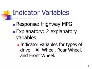
7.1 Using and Interpreting Indicator Variables • Suppose some observations have a particular characteristic or attribute, while others do not. • We can include this information in the regression model by using dummy or indicator variables. Indicator Variables
Add the info thru a coding scheme Use a binary (dummy) variable to “indicate” when the characteristic is present Di = 1 if observation i has the attribute Di = 0 if observation i does not have it Indicator Variables
An Example Di = 1 if individual i is employed Di = 0 if individual i is not employed We could do it the other way and use the "1" to indicate an unemployed individual. Indicator Variables
Multiple Categories • For multiple categories, use multiple indicators. • For example, to indicate where a firm's stock is listed, we could define 3 indicator variables; one each for the NYSE, AMEX and NASDAQ. • For computational reasons, we would include only two of these in the regression. Indicator Variables
Example 7.1 Employment Discrimination If two groups have apparently different salary structures, you first need to account for differences in education, training and experience before any claim of discrimination can be made. Regression analysis with an indicator variable for the group is a way to investigate this. Indicator Variables
Treasury Versus Harris The data set HARRIS7 contains information on the salaries of 93 employees of the Harris Trust and Savings Bank. They were sued by the US Department of Treasury in 1981. Here we examine how salary depends on education, also accounting for gender. Indicator Variables
Salary Versus Years of Education At all levels of education, the male salaries appear higher. Indicator Variables
Regression Analysis The regression equation is SALARY = 4173 + 80.7 EDUCAT + 692 MALES Predictor Coef SE Coef T P Constant 4173.1 339.2 12.30 0.000 EDUCAT 80.70 27.67 2.92 0.004 MALES 691.8 132.2 5.23 0.000 S = 572.4 R-Sq = 36.3% R-Sq(adj) = 34.9% How do we interpret this equation? Indicator Variables
An Intercept Adjuster For an indicator variable, the bj is not really a slope. To see this, evaluate the equation for the two groups. FEMALES (MALES = 0) SALARY = 4173 + 80.7 EDUCAT + 692 MALES = 4173 + 80.7 EDUCAT + 692 (0) = 4173 + 80.7 EDUCAT MALES (MALES = 1) SALARY = 4173 + 80.7 EDUCAT + 692 MALES = 4173 + 80.7 EDUCAT + 692 (1) = 4173 + 80.7 EDUCAT + 692 = 4865 + 80.7 EDUCAT Indicator Variables
Parallel Salary Equations Indicator Variables
H0: MALES = 0 Ha: MALES ≠ 0 Use t = b/SEb as usual t = 5.23 is significant (After accounting for years of education, there is no salary difference) (After accounting for education, there IS a salary difference) Is The Difference Significant? Indicator Variables
What if the Coding Was Different? • If we had an indicator for females and used it, the equation would be: SALARY = 4865 + 80.7 EDUCAT - 692 FEMALES • The difference between the groups is the same. For females, the intercept in the equation is 4865 – 692 = 4173 Indicator Variables
Multiple Categories • Pick one category as the "base category". • Create one indicator variable for each other category. • In general, if there are m categories, use m – 1 indicator variables. Indicator Variables
Example 7.3 Meddicorp Sales Y = Sales in one of 25 territories X1 = advertising in territory X2 = bonuses paid in territory Also Region: 1 = South 2 = West 3 = Midwest Indicator Variables
How do you use region? What happens if you just put it in the model? Sales = -84 + 1.55 ADV + 1.11 BONUS + 119 Region R2 = 92.0% and Se = 68.89 SE(Region) = 28.69 so tstat = 4.14 is significant Indicator Variables
Region as an X This implies the difference between Region 3 (MW) and Region 2 (W) = b3 = 119 And the difference between Region 2 (W) and Region 1 (S) is also 119 The sales differences may not be equal but this forces them to be estimated that way Indicator Variables
A more flexible approach • Use two indicator variables to tell the three regions apart • Can use any one of the three as the “base” category. • Here is what it looks like if Midwest is selected as the base. Indicator Variables
Coding scheme 1 0 0 0 1 0 Indicator Variables
Results SALES = 435 + 1.37ADV + .975 BONUS - 258 South – 210 West R2 = 94.7 and Se = 57.63 Both indicators are significant Indicator Variables
This Defines Three Equations SALES = 435 + 1.37ADV + .975 BONUS - 258 South – 210 West S: SALES = 177 + 1.37ADV + .975 BONUS W: SALES = 225 + 1.37ADV + .975 BONUS MW: SALES = 435 + 1.37ADV + .975 BONUS Indicator Variables
Is Location Significant? • Because location is measured by two variables in a group, we need to do a partial F test. • The full Model has ADV, BONUS, SOUTH and WEST and has R2 = 94.7 • The reduced model has only ADV and BONUS, with R2 = 85.5 Indicator Variables
Output For F-Test FULL MODEL S = 57.63 R-Sq = 94.7% R-Sq(adj) = 93.6% Analysis of Variance Source DF SS MS F P Regression 4 1182560 295640 89.03 0.000 Residual Error 20 66414 3321 Total 24 1248974 REDUCED MODEL S = 90.75 R-Sq = 85.5% R-Sq(adj) = 84.2% Analysis of Variance Source DF SS MS F P Regression 2 1067797 533899 64.83 0.000 Residual Error 22 181176 8235 Total 24 1248974 Indicator Variables
Partial F Computations (SSER – SSEF) / (K – L) F = MSEF (181176 - 66414)/ (4-2) = = 17.3 3321 Indicator Variables
7.2 Interaction Variables • Another type of variable used in regression models is an interaction variable. • This is usually formulated as the product of two variables; for example, x3 = x1x2 • With this variable in the model, it means the level of x2changes how x1affects Y Indicator Variables
Interaction Model With two x variables the model is: If we factor out x1we get: so each value of x2 yields a different slope in the relationship between y and x1 Indicator Variables
Interaction Involving an Indicator If one of the two variables is binary, the interaction produces a model with two different slopes. When x2 = 0 When x2 = 1 Indicator Variables
Example 7.4 Discrimination (again) • In the Harris Bank case, suppose we suspected that the salary difference by gender changed with different levels of education. • To investigate this, we created a new variable MSLOPE = EDUCAT*MALES and added it to the model. Indicator Variables
Regression Output The regression equation is SALARY = 4395 + 62.1 EDUCAT - 275 MALES + 73.6 MSLOPE Predictor Coef SE Coef T P Constant 4395.3 389.2 11.29 0.000 EDUCAT 62.13 31.94 1.95 0.055 MALES -274.9 845.7 -0.32 0.746 MSLOPE 73.59 63.59 1.16 0.250 S = 571.4 R-Sq = 37.3% R-Sq(adj) = 35.2% How do we interpret the equation this time? Indicator Variables
A Slope Adjuster To see the interaction effect, once again evaluate the equation for the two groups. FEMALES (MALES = 0) SALARY = 4395 + 62.1 EDUCAT - 275 MALES + 73.6 MSLOPE = 4395 + 62.1 EDUCAT - 275 (0) + 73.6 (EDUCAT*0) = 4395 + 62.1 EDUCAT MALES (MALES = 1) SALARY = 4395 + 62.1 EDUCAT - 275 MALES + 73.6 MSLOPE = 4395 + 62.1 EDUCAT - 275 (1) + 73.6 (EDUCAT*1) = 4395 + 62.1 EDUCAT – 275 + 73.6 EDUCAT = 4120 + 135.7 EDUCAT Indicator Variables
Lines With Two Different Slopes A bigger gap occurs at higher education levels Indicator Variables
Tests in This Model • Although the slope adjuster implies the salary gap increases with education, this effect is not really significant (tMSLOPE = 1.16). • The overall affect of gender is now contained in two variables, so a partial F test would be needed to test for differences between male and female salaries. Indicator Variables
7.3 Seasonal Effects in Time Series Regression • Data collected over time (say quarterly) • If we think the Y variable depends on the calendar can do a kind of “seasonal adjustment” by adding quarter dummies • Q1 = 1 if this was first quarter, Q2 = 1 if a second quarter, Q3 = 1 if third • Don’t use Q4 since that is the “base” Indicator Variables
Example 7.5 ABX Company Sales • We fit a trend to these sales in Example 3.11 by regressing sales on a time index variable. • Because this company sells winter sports merchandise, including seasonal effects should markedly improve the fit. Indicator Variables
ABX Company Sales 4th qtr Indicator Variables
Two Regressions The regression equation is SALES = 199 + 2.56 TIME Predictor Coef SE Coef T P Constant 199.017 5.128 38.81 0.000 TIME 2.5559 0.2180 11.73 0.000 S = 15.91 R-Sq = 78.3% R-Sq(adj) = 77.8% The regression equation is SALES = 211 + 2.57 TIME + 3.75 Q1 - 26.1 Q2 - 25.8 Q3 Predictor Coef SE Coef T P Constant 210.846 3.148 66.98 0.000 TIME 2.56610 0.09895 25.93 0.000 Q1 3.748 3.229 1.16 0.254 Q2 -26.118 3.222 -8.11 0.000 Q3 -25.784 3.217 -8.01 0.000 S = 7.190 R-Sq = 95.9% R-Sq(adj) = 95.5% Indicator Variables
Are the Seasonal Effects Significant? • The strong t-ratios for Q2 and Q3 say "yes" and the model R2 increased by 17.6% when we added the seasonal indicators. • With evidence this strong we probably don't need to test further. • In general, however, we would need another partial F test to see if the overall seasonal effect is significant. Indicator Variables