Download
1 / 27
270 likes | 447 Views
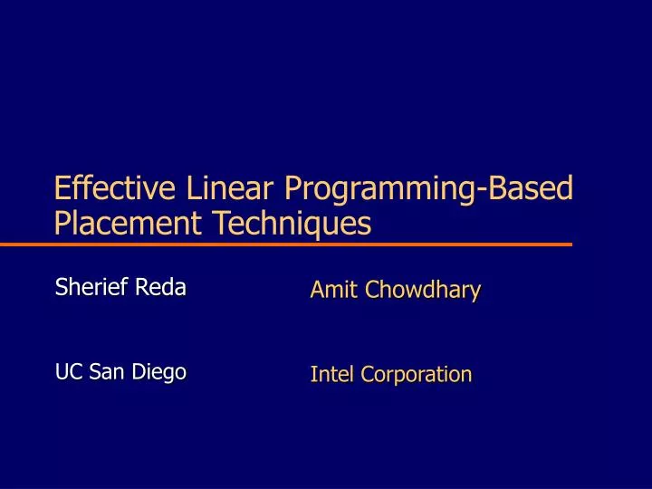
Effective Linear Programming-Based Placement Techniques. Sherief Reda UC San Diego. Amit Chowdhary Intel Corporation. Outline. Motivation Modeling of cell spreading Linear programming (LP)-based placer Applications of LP-based placer Experimental results Conclusions. Motivation.

E N D
Effective Linear Programming-Based Placement Techniques Sherief Reda UC San Diego Amit Chowdhary Intel Corporation
Outline • Motivation • Modeling of cell spreading • Linear programming (LP)-based placer • Applications of LP-based placer • Experimental results • Conclusions
Motivation • Linear programming has been shown to be effective in modeling timing objective during placement • Static timing can be modeled as linear constraints using the notion of differential timing [DAC 2005] • Linear programming can effectively model wirelength as half-perimeter wirelength (HPWL) • Cell spreading not modeled in linear programming yet • LP has been restricted to incremental placement
Main Contribution • In this paper, we model cell spreading using linear constraints • Designed a global placer based on linear programming • Efficient modeling of timing and wirelength • Uses relative placement constraints to spread cells gradually • Our LP-based placement approach can be used as • Global placer • Whitespace allocator (WSA)
LP-based Placement Approach • Place cells using an ideal or exact HPWL model of wirelength • Use this initial placement to establish a relative ordering of cells • Transform relative order of cells into linear constraints • Solve the corresponding LP problem to spread cells while maintaining relative order • Iterate till cells are spread out
Placement after iteration 2 Placement after iteration 3 Placement after iteration 4 Legalized placement LP-based Placement Approach Placement after iteration 1 Initial WL-optimal placement
uppery Net lowery rightx leftx Modeling of wirelength • leftx, rightx, lowery and uppery variables defined for every net • HPWL model of wirelength used • For every cell at location (x,y)connected to net • Length of this net is
Lower bound on wirelength • Length of a net has a lower bound based on the area of cells connected to it • Lower bound on each net spreads out cells • Helps in defining relative order of cells • Overall wirelength objective is
Modeling of timing • Various aspects of static timing analysis can be formulated as linear constraints of cell placements [DAC2005] • Delay and transition time for cells • Delay and transition time for nets • Propagated arrival times • Slack at cell pins • Timing metrics • worst negative slack WNS • total negative slack TNS
Defining relative order • For each cell v, define four sets corresponding to the cells to the left, right, upper, and below v • Quadratic time and space complexity • Reduce space complexity to linear using transitivity • Still quadratic time • We use fast heuristic methods that capture a good amount of the relative order relationships • Q-adjacency graph • Delaunay triangulation
Q-adjacency Graph • Simple Idea: Establish an adjacency between each cell and its closest cell in each of the four quadrant • Complexity is O(M.logM + k.M), where k is a constant that depends on the input placement
Delaunay Triangulation • Capture adjacency using Delaunay triangulation Delaunay triangulation (dual of the Voronoi diagram) Voronoi diagram • Voronoi diagram • Partitioning of a plane with n points into convex polygons such that each polygon contains exactly one generating point and every point in a given polygon is closer to itsgenerating point than to any other point
Q-ADJ Q-ADJ+ DEL DEL Example of Delaunay and Q-Adjacency • We use relative order from Q-Adjacency as well as Delaunay triangulation
v u v u v u LP Modeling of Relative Order For each adjacency {u, v}: 1. if u and v overlap in the current placement then next separation = current separation + minimum additional separation to remove the overlap and make sure u and v relative positions stay the same • make sure the amount of overlap reduces 2. if u and v do not overlap • make sure a non-overlap does not turn into an overlap
LP-Based Placement Techniques • Our LP-based placement approach can be used in several ways • Wirelength-driven global placement • Whitespace allocation • Timing- and wirelength-driven global placement
Unplaced circuit Relative Placement MidX - Spreading Legalization Detailed Placement Final Placement 1. Wirelength-driven Global Placement
Benchmark statistics • Circuits chosen from a recent microprocessor
Comparison with Other Placers • Compared results with other placers • Capo 9.3 (UMich) • Better of FengShui 2.6 and 5.1 (SUNY) • APlace 2.0 (UCSD) • Better of mPL 4.1 and 5.0 (UCLA) • All placements were measured using the same HPWL calculator
Placements of different placers APlace2.0 mPL5.0 Our Placement HPWL = 881 HPWL = 802 FengShui5.1 Capo9.3 HPWL = 804 HPWL = 891 HPWL = 823
2. Whitespace Allocation • In an existing legal placement, we redistribute white space to optimize wirelength Unplaced circuit Global Placement + Legalization MidX – Whitespace Allocation Legalization Detailed Placement Final Placement
Input global placement: HPWL = 9.43 After MidX: HPWL = 8.76 After MidX and legalization: HPWL = 8.81 Whitespace Allocation: Example
Unplaced circuit Timing-optimal Relaxed Placement MidXT - Spreading Legalization Detailed Placement Final Placement 3. Timing-driven global placement
Timing-driven global placement • Start with a timing-optimal relaxed placement obtained using our differential timing-based placer [DAC 2005] • Identify timing critical cells from a static timer • Spread cells using MidXT with a combined objective of • Minimize total wirelength of all nets • Minimize total displacement of all timing-critical cells • We are working on integrating the static timing constraints in MidXT placer
After MidXT: TNS = -9.40 After legalization: TNS = -10.34 Timing-driven placement: Example Input Placement: TNS = -13.99 Relaxed placement: TNS = -8.82
Conclusions • Extended LP-based placement approach to model cell spreading • Relative order amongst adjacent cells are transformed into linear constraints • Presented a powerful LP-based global placer • Gradually spreads cells while maintaining relative order • Benchmarked against academic placers • Models timing and wirelength very accurately